Note
Go to the end to download the full example code
Electrical resistivity tomography#
What we do in this notebook#
Here we look at applying CoFI to an electrical resistivity tomography problem, and explore different iterative non linear solvers.
Learning outcomes#
A demonstration of CoFI’s ability to interface with PyGIMLi (Geophysical Inversion and Modelling Library), a mature package to solve the ERT forward problem
An exposé of CoFI’s ability to interface with the iterative non-linear solvers in SciPy specifically
scipy.optimizeand PyTorch specificiallytorch.optimAn illustration of how CoFI can be used to identify the most appropriate iterative non-linear solver for a given problem
# Environment setup (uncomment code lines below)

# !pip install -U cofi geo-espresso

# !pip install -q condacolab
# import condacolab
# condacolab.install()
# !mamba install -c gimli pygimli=1.3
If you see a warning message from Colab - don’t worry, this is expected. This happens when we’ve successfully installed a package manager (“mamba”) so that we can then install PyGIMLi (from conda channel “gimli”).

Remember to uncomment and run the code cell below as well, as we are going to load some data from GitHub.
# !git clone https://github.com/inlab-geo/cofi-examples.git
# %cd cofi-examples/tutorials/
Problem description#
Electrical resistivity tomography is the inversion of measurements of apparent electrical resistivities measured between electrodes placed at the surface. A measured/known current is applied to one electrode pair and a second electrode pair is used to measure the voltage, this then allows to compute an apparent resistivity between the two electrode pairs. Its applications include the detection and delineation of groundwater resources, fracture zones, clay formations and the monitoring of pollution plumes.
Here we illustrate the expandability of CoFI by combining a mature Python library for geophysical inversion that implements one iterative non-linear inversion method (Newton step with line search) for ERT (PyGIMLI https://www.pygimli.org/) with the iterative non linear solvers we have made available in CoFI. In the following the forward problem will be solved using PyGIMLI, while the inverse problem will be solved using CoFI.
The objective function we are minimizing is given as:
where \(\mathbf{d}\) represents the data vector of measured apparent resistivties, \(\mathrm{f}(\mathbf{m})\) is the model prediction, \(C_d^{-1}\) is the inverse of the data covariance matrix, \(W\) the model smoothing matrix, \(\mathbf{m}\) the model vector and \(\lambda\) a regularization factor.
The model update is then given as
where \(J\) represents the Jacobian.
Successful inversion also relies on the objective function being smooth and predictable. For apparent resistivity data it is advantageous to convert measurements and model parameters to scale logarithmically to obtain a smoother and more predictable objective function when compared with using the unscaled data and unscaled model parameters.
Further reading#
Rücker, C., Günther, T., & Spitzer, K. (2006). Three-dimensional modelling and inversion of dc resistivity data incorporating topography – I. Modelling. Geophys. J. Int, 166, 495–505. https://doi.org/10.1111/j.1365-246X.2006.03010.x
Günther, T., Rücker, C., & Spitzer, K. (2006). Three-dimensional modelling and inversion of dc resistivity data incorporating topography - II. Inversion. Geophysical Journal International, 166(2), 506–517. https://doi.org/10.1111/J.1365-246X.2006.03011.X
Wheelock, B., Constable, S., & Key, K. (2015). The advantages of logarithmically scaled data for electromagnetic inversion. Geophysical Journal International, 201(3), 1765–1780. https://doi.org/10.1093/GJI/GGV107
Interfacing to PyGIMLi#
PyGIMLi provides all the functionality to compute the apparent resistivities and Jacobian given a model. One of our goals around CoFI is to never reinvent the wheel and thus in the following we will - rely on PyGIMLi’s functionality to plot the model and data; and - use PyGIMLi’s capabilities to compute the response and the Jacobian from a model.
To achieve this we first define a set of utility functions that will facilitate interfacing to PyGIMLi. We will also show how CoFI can directly interface with a mature package without the need to go via Espresso.
PyGIMLi uses different meshes and adaptive meshing capabilities via Gmsh https://gmsh.info/, all CoFI needs to access are the model vector, the Jacobian, the regularization matrix and the model prediction. This makes for a minimal interface.
import numpy as np
import matplotlib.pyplot as plt
import matplotlib as mpl
import pygimli
from pygimli.physics import ert
from pygimli import meshtools

from cofi import BaseProblem, InversionOptions, Inversion

np.random.seed(42)
#@title utility functions (hidden)
############# Utility functions using PyGIMLi ##############################################

# inversion mesh bound
x_inv_start = -5
x_inv_stop = 55
y_inv_start = -20
y_inv_stop = 0
x_invmesh = np.linspace(start=x_inv_start, stop=x_inv_stop, num=40)
y_invmesh = np.linspace(start=y_inv_start,stop=y_inv_stop,num=10)

# Dipole Dipole (dd) measuring scheme
def survey_scheme(start=0, stop=50, num=51, schemeName="dd"):
    scheme = ert.createData(elecs=np.linspace(start=start, stop=stop, num=num),schemeName=schemeName)
    return scheme

# true geometry, forward mesh and true model
def model_true(scheme, start=[-55, 0], end=[105, -80], anomaly_pos=[10,-7], anomaly_rad=5):
    world = meshtools.createWorld(start=start, end=end, worldMarker=True)
    for s in scheme.sensors():          # local refinement
        world.createNode(s + [0.0, -0.1])
    conductive_anomaly = meshtools.createCircle(pos=anomaly_pos, radius=anomaly_rad, marker=2)
    geom = world + conductive_anomaly
    rhomap = [[1, 200], [2,  50],]
    mesh = meshtools.createMesh(geom, quality=33)
    return mesh, rhomap

# PyGIMLi ert.ERTManager
def ert_manager(data, verbose=False):
    return ert.ERTManager(data, verbose=verbose, useBert=True)

# inversion mesh
def inversion_mesh(ert_mgr):
    inv_mesh = ert_mgr.createMesh(ert_mgr.data)
    # print("model size", inv_mesh.cellCount())   # 1031
    ert_mgr.setMesh(inv_mesh)
    return inv_mesh

# inversion mesh rectangular (the above is by default triangular)
def inversion_mesh_rect(ert_manager):
    inv_mesh = pygimli.createGrid(x=x_invmesh, y=y_invmesh, marker=2)
    inv_mesh = pygimli.meshtools.appendTriangleBoundary(inv_mesh, marker=1, xbound=50, ybound=50)
    # print("model size", inv_mesh.cellCount())    # 1213
    ert_manager.setMesh(inv_mesh)
    return inv_mesh

# PyGIMLi ert.ERTModelling
def ert_forward_operator(ert_manager, scheme, inv_mesh):
    forward_operator = ert_manager.fop
    forward_operator.setComplex(False)
    forward_operator.setData(scheme)
    forward_operator.setMesh(inv_mesh, ignoreRegionManager=True)
    return forward_operator

# regularization matrix
def reg_matrix(forward_oprt):
    region_manager = forward_oprt.regionManager()
    region_manager.setConstraintType(2)
    Wm = pygimli.matrix.SparseMapMatrix()
    region_manager.fillConstraints(Wm)
    Wm = pygimli.utils.sparseMatrix2coo(Wm)
    return Wm

# initialise model
def starting_model(ert_mgr, val=None):
    data = ert_mgr.data
    start_val = val if val else np.median(data['rhoa'].array())     # this is how pygimli initialises
    start_model = np.ones(ert_mgr.paraDomain.cellCount()) * start_val
    start_val_log = np.log(start_val)
    start_model_log = np.ones(ert_mgr.paraDomain.cellCount()) * start_val_log
    return start_model, start_model_log

# convert model to numpy array
def model_vec(rhomap, fmesh):
    model_true = pygimli.solver.parseArgToArray(rhomap, fmesh.cellCount(), fmesh)
    return model_true

# plot colorbar for model
def colorbar_model(ax, init=False, orientation="horizontal"):
    val_min = 170 if init else rhomap[1][1]
    val_max = 230 if init else rhomap[0][1]
    norm = mpl.colors.Normalize(val_min, val_max)
    sm = plt.cm.ScalarMappable(norm=norm)
    cb = plt.colorbar(sm, orientation=orientation, ax=ax)
    cb.set_label(r'$\Omega \mathrm{m}$')
    cb.set_ticks(np.arange(val_min, val_max+1, 30))

# plot colorbar for data
def colorbar_data(ax, orientation="horizontal"):
    norm = mpl.colors.Normalize(min(data["rhoa"]), max(data["rhoa"]))
    sm = plt.cm.ScalarMappable(norm=norm)
    cb = plt.colorbar(sm, orientation=orientation, ax=ax)
    cb.set_label(r'$\Omega \mathrm{m}$')
    cb.set_ticks(np.arange(min(data["rhoa"]), max(data["rhoa"]), 30))

# plot true model, inferred model, provided data and synthetic data from inv_result
def plot_result(inv_result, title=None):
    # convert back to normal space from log space
    model = np.exp(inv_result.model)

    fig, axes = plt.subplots(1, 2, figsize=(12,4))
    if title is not None:
        fig.suptitle(title, fontsize=16)

    # plot inferred model
    # inv_result.summary()
    pygimli.show(ert_mgr.paraDomain, data=model, label=r"$\Omega m$", ax=axes[0], cMax=rhomap[0][1], cMin=rhomap[1][1], colorBar=False)
    axes[0].set_title("Inferred model")
    axes[0].set_xlabel("Horizontal Distance (m)")
    axes[0].set_ylabel("Elevation (m)")

    # plot the true model
    pygimli.show(mesh, data=rhomap, label="$\Omega m$", showMesh=True, ax=axes[1], colorBar=False)
    axes[1].set_xlim(x_inv_start, x_inv_stop)
    axes[1].set_ylim(y_inv_start, y_inv_stop)
    axes[1].set_title("True model")
    axes[1].set_xlabel("Horizontal Distance (m)")
    colorbar_model(axes, orientation="vertical")

    # plot the data
    _, axes = plt.subplots(1, 2, figsize=(12,4))

    # plot synthetic data
    d = forward_oprt.response(model)
    ert.show(scheme, vals=d, cMin=np.min(data["rhoa"]), cMax=np.max(data["rhoa"]), ax=axes[0], colorBar=False)
    axes[0].set_title("Synthetic data from inferred model")
    axes[0].set_xlabel("Horizontal Distance (m)")
    axes[0].set_ylabel("Dipole Dipole Separation (m)")
    # plot given data
    ert.show(data, ax=axes[1], colorBar=False)
    axes[1].set_title("Provided data")
    axes[1].set_xlabel("Horizontal Distance (m)")
    colorbar_data(axes, orientation="vertical")
True model#
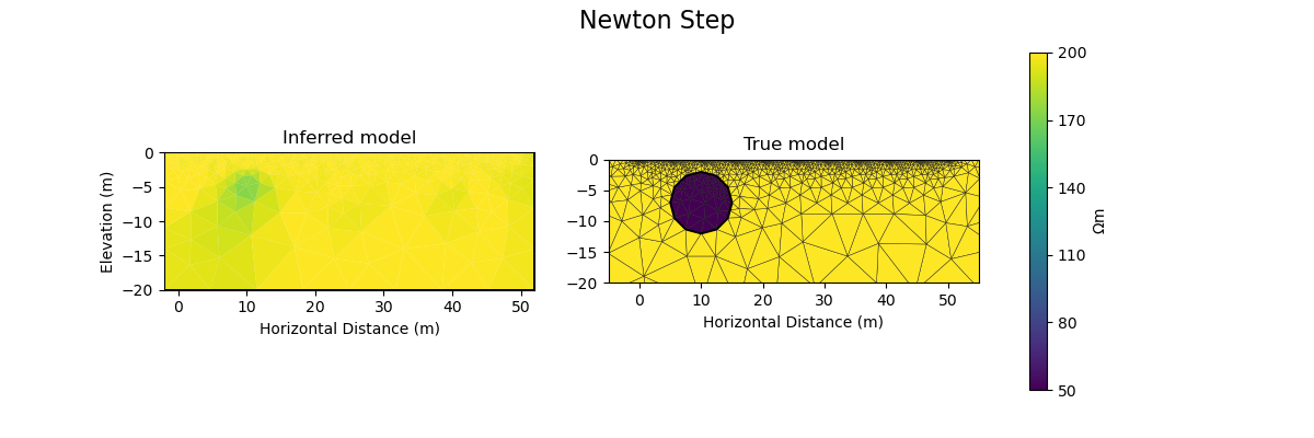
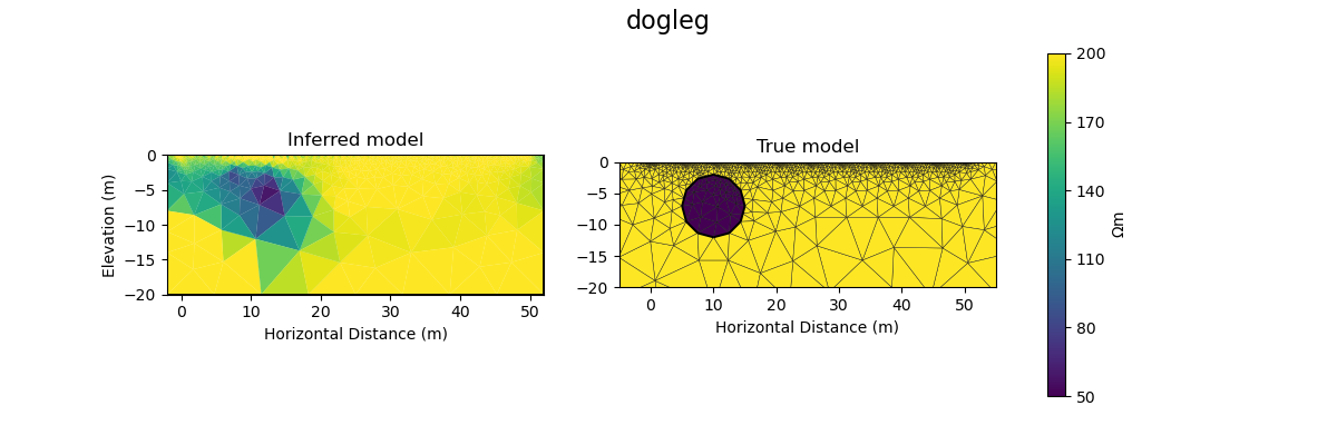
Our example is centred around inverting dipole dipole measurements of apparent resistivities in 2D with a circular shaped low resistivity anomaly.
Further reading#
https://www.agiusa.com/dipole-dipole%E2%80%8B-%E2%80%8Barray%E2%80%8B
# PyGIMLi - define measuring scheme, geometry, forward mesh and true model
scheme = survey_scheme()
mesh, rhomap = model_true(scheme)

# plot the true model
_, ax = plt.subplots(figsize=(10,8))
pygimli.show(mesh, data=rhomap, label="$\Omega \mathrm{m}$", showMesh=True, ax=ax, colorBar=False)
ax.set_xlim(x_inv_start, x_inv_stop)
ax.set_ylim(y_inv_start, y_inv_stop)
ax.set_title("True model")
ax.set_xlabel("Horizontal Distance (m)")
ax.set_ylabel("Elevation (m)")
colorbar_model(ax)
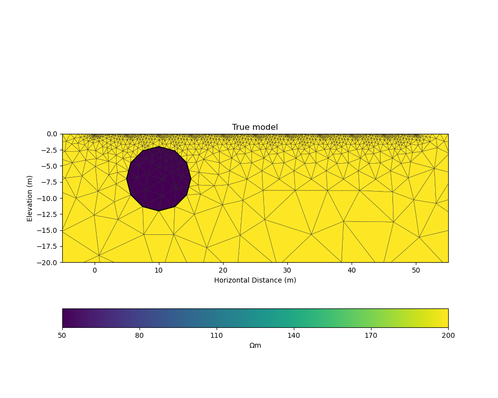
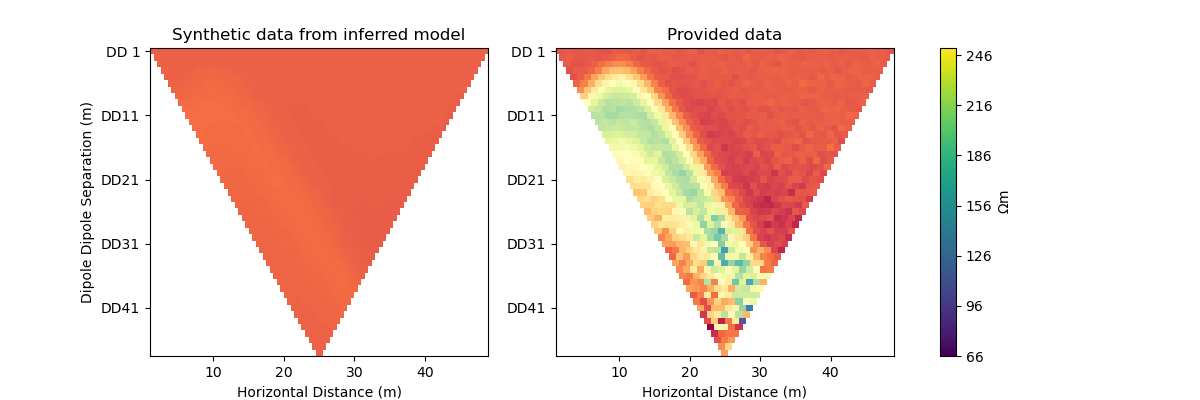
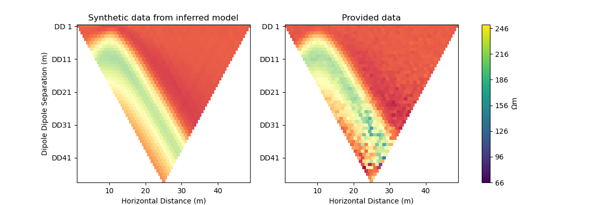
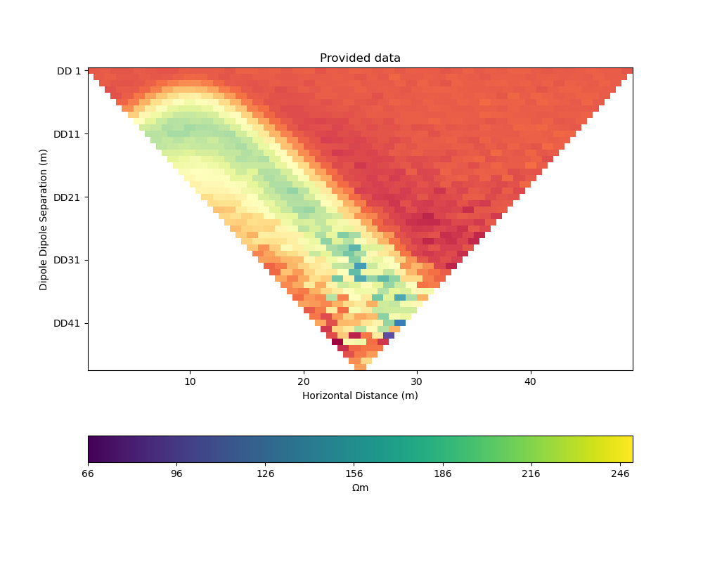
ERT measurements consist of the apparent resistivity measured between multiple electrode pairs and they are commonly plotted as pseudosections. The model response for the true model has been previously computed with PyGIMLi and noise has been added with the magnitude of the noise depending on the dipole dipole separation.
# load data and covariance matrix
log_data = np.loadtxt("ert_data_log.txt")
data_cov_inv = np.loadtxt("ert_data_cov_inv.txt")

# create PyGIMLi's ERT manager
ert_mgr = ert_manager("ert_data.dat")
# plot data
data = ert_mgr.data
_, ax = plt.subplots(figsize=(10,8))
ert.show(data, ax=ax, colorBar=False)
ax.set_title("Provided data")
ax.set_xlabel("Horizontal Distance (m)")
ax.set_ylabel("Dipole Dipole Separation (m)")
colorbar_data(ax)
Forward operator#
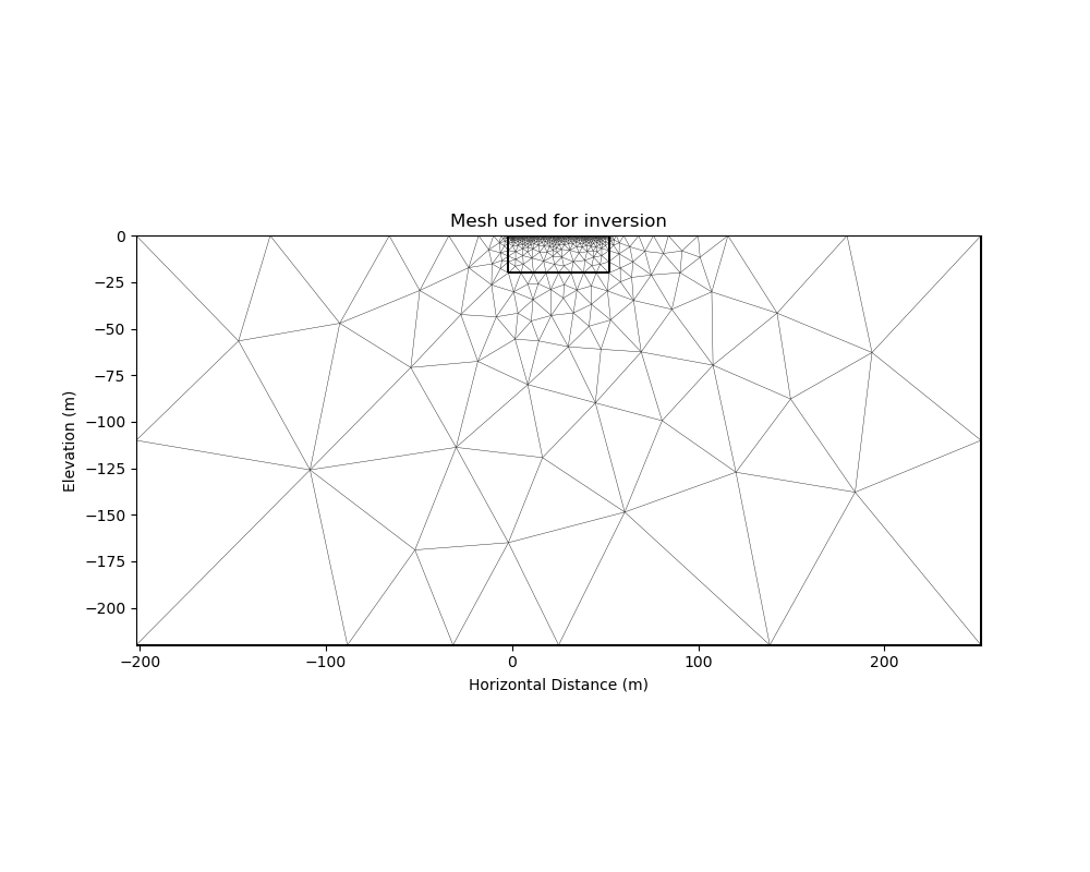
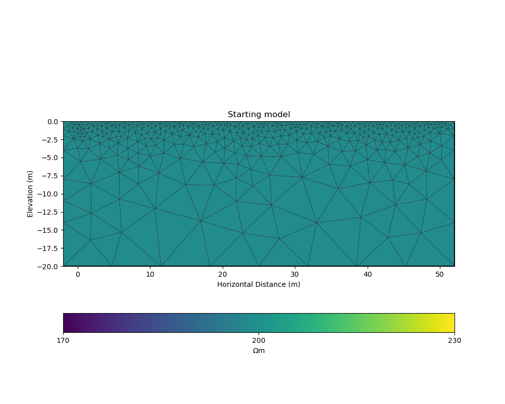
PyGIMLi solves the ERT forward problem accurately and efficiently by defining boundary cells or ghost cells around the region of interest and creating an optimal triangular mesh. This is all handled by PyGIMLi and Gmsh and the model vector for the purpose of the inversion are the cells plotted in yellow.
inv_mesh = inversion_mesh(ert_mgr)
_, ax = plt.subplots(figsize=(10,8))
pygimli.show(inv_mesh, showMesh=True, markers=False, colorBar=False, ax=ax)
ax.set_title("Mesh used for inversion");
ax.set_xlabel("Horizontal Distance (m)");
ax.set_ylabel("Elevation (m)");
Text(71.47222222222221, 0.5, 'Elevation (m)')
# PyGIMLi's forward operator (ERTModelling)
forward_oprt = ert_forward_operator(ert_mgr, scheme, inv_mesh)

# extract regularisation matrix
Wm = reg_matrix(forward_oprt)

# initialise a starting model for inversion
start_model, start_model_log = starting_model(ert_mgr)
_, ax = plt.subplots(figsize=(10,8))
pygimli.show(ert_mgr.paraDomain, data=start_model, label="$\Omega m$", showMesh=True, colorBar=False, cMin=170, cMax=230, ax=ax)
ax.set_title("Starting model")
ax.set_xlabel("Horizontal Distance (m)");
ax.set_ylabel("Elevation (m)");
colorbar_model(ax, init=True)
The next step is to define the functions for CoFI. Typically, a given inversion solver will only require a subset of the functions we define in the following but in this example we would like to explore a wide range of solvers.
#@title additional utility functions (hidden)
############# Functions provided to CoFI ##############################################

## Note: all functions below assume the model in log space!

def _ensure_numpy(model):
    if "torch.Tensor" in str(type(model)):
        model = model.cpu().detach().numpy()
    return model

def get_response(model, forward_operator):
    model = _ensure_numpy(model)
    return np.log(np.array(forward_operator.response(np.exp(model))))

def get_residual(model, log_data, forward_operator):
    response = get_response(model, forward_operator)
    residual = log_data - response
    return residual

def get_jacobian(model, forward_operator):
    response = get_response(model, forward_operator)
    model = _ensure_numpy(model)
    forward_operator.createJacobian(np.exp(model))
    J = np.array(forward_operator.jacobian())
    jac = J / np.exp(response[:, np.newaxis]) * np.exp(model)[np.newaxis, :]
    return jac

def get_jac_residual(model, log_data, forward_operator):
    response = get_response(model, forward_operator)
    residual = log_data - response
    model = _ensure_numpy(model)
    forward_operator.createJacobian(np.exp(model))
    J = np.array(forward_operator.jacobian())
    jac = J / np.exp(response[:, np.newaxis]) * np.exp(model)[np.newaxis, :]
    return jac, residual

def get_data_misfit(model, log_data, forward_operator, data_cov_inv=None):
    residual = get_residual(model, log_data, forward_operator)
    data_cov_inv = np.eye(log_data.shape[0]) if data_cov_inv is None else data_cov_inv
    return np.abs(residual.T @ data_cov_inv @ residual)

def get_regularization(model, Wm, lamda):
    model = _ensure_numpy(model)
    model = np.exp(model)
    return lamda * (Wm @ model).T @ (Wm @ model)

def get_objective(model, log_data, forward_operator, Wm, lamda, data_cov_inv=None):
    data_misfit = get_data_misfit(model, log_data, forward_operator, data_cov_inv)
    regularization = get_regularization(model, Wm, lamda)
    obj = data_misfit + regularization
    return obj

def get_gradient(model, log_data, forward_operator, Wm, lamda, data_cov_inv=None):
    jac, residual = get_jac_residual(model, log_data, forward_operator)
    data_cov_inv = np.eye(log_data.shape[0]) if data_cov_inv is None else data_cov_inv
    data_misfit_grad =  - residual.T @ data_cov_inv @ jac
    regularization_grad = lamda * Wm.T @ Wm @ np.exp(model)
    return data_misfit_grad + regularization_grad

def get_hessian(model, log_data, forward_operator, Wm, lamda, data_cov_inv=None):
    jac = get_jacobian(model, forward_operator)
    data_cov_inv = np.eye(log_data.shape[0]) if data_cov_inv is None else data_cov_inv
    hess = jac.T @ data_cov_inv @ jac + lamda * Wm.T @ Wm
    return hess
CoFI BaseProblem#
As in the traveltime tomography example, we now use these functions to
define our BaseProblem.
# hyperparameters
lamda = 0.0001

# CoFI - define BaseProblem
ert_problem = BaseProblem()
ert_problem.name = "Electrical Resistivity Tomography defined through PyGIMLi"
ert_problem.set_forward(get_response, args=[forward_oprt])
ert_problem.set_jacobian(get_jacobian, args=[forward_oprt])
ert_problem.set_residual(get_residual, args=[log_data, forward_oprt])
ert_problem.set_data_misfit(get_data_misfit, args=[log_data, forward_oprt, data_cov_inv])
ert_problem.set_regularization(get_regularization, args=[Wm, lamda])
ert_problem.set_gradient(get_gradient, args=[log_data, forward_oprt, Wm, lamda, data_cov_inv])
ert_problem.set_hessian(get_hessian, args=[log_data, forward_oprt, Wm, lamda, data_cov_inv])
ert_problem.set_initial_model(start_model_log)
With the BaseProblem defined, we can ask CoFI to list the solver
libraries we can use for our problem.
ert_problem.suggest_tools();
Based on what you've provided so far, here are possible tools:
{
    "optimization": [
        "scipy.optimize.minimize",
        "scipy.optimize.least_squares",
        "torch.optim"
    ],
    "matrix solvers": [
        "cofi.simple_newton"
    ],
    "sampling": [
        "bayesbay",
        "neighpy"
    ]
}

{'optimization': ['scipy.optimize.minimize', 'scipy.optimize.least_squares', 'torch.optim'], 'matrix solvers': ['cofi.simple_newton'], 'sampling': ['bayesbay', 'neighpy']}
From the traveltime tomography example we know that the
cofi.simple_newton solver worked well so we will try it.
Newton step#
The Jacobian and Hessian are only local measures of the first and second derivatives of the objective function and given the ERT inverse problem is non-linear, we can no longer take the full Newton step to compute a model update. In practice:
If the step length is chosen too large we may end up with a model that is non-physical and the forward solver will crash and/or we will overshoot.
If the step size is chosen too small too many iterations might be needed to reach convergence
inv_options_newton = InversionOptions()
inv_options_newton.set_tool("cofi.simple_newton")
inv_options_newton.set_params(num_iterations=5, step_length=0.01)

inv = Inversion(ert_problem, inv_options_newton)
inv_result = inv.run()
# inv_result.summary()
print(f"\nNumber of objective function evaluations: {inv_result.n_obj_evaluations}")
print(f"Number of gradient function evaluations: {inv_result.n_grad_evaluations}")
print(f"Number of hessian function evaluations: {inv_result.n_hess_evaluations}")

plot_result(inv_result, "Newton Step")
Iteration #0, updated objective function value: 224.79875151413356
Iteration #1, updated objective function value: 220.3623726879779
Iteration #2, updated objective function value: 215.90570020911244
Iteration #3, updated objective function value: 211.6177561325534
Iteration #4, updated objective function value: 207.38256930187458

Number of objective function evaluations: 6
Number of gradient function evaluations: 5
Number of hessian function evaluations: 5
Convergence of Newton’s Method - A pathological example#
A simple illustrative example of the limitations around Newton’s method is finding the \(x\) where \(f(x)=0\) for the following non-convex function:
\(f(x) = x^3 − 2x + 2\), with \(\nabla f(x) = 3x^2 -2\) and $H_f(x) = 6 x $
If we start with \(x=0\) or \(x=1\) the result will oscillate between 0 and 1 and never converge to the correct solution of \(x\approx -1.77\)
Further reading#
import scipy
x0=0.1
scipy.optimize.newton(lambda x: x**3-2*x+2, x0, fprime=lambda x: 3 * x**2-2,
                       fprime2=lambda x: 6 * x,full_output=True, disp=True,maxiter=51)
(-1.7692923542386314,       converged: True
           flag: converged
 function_calls: 39
     iterations: 13
           root: -1.7692923542386314
         method: halley)
PyGIMLi uses a line search to determine the optimal step length, that means the descent direction is given by the full Newton Step with the length adjusted so that it does not overshoot and results in an improvement of the fit to the data. The major alternative to employing a line search is to employ a trust region method. Trust regions methods try to estimate the region around the current model within which the assumption of local linearity holds and then limit the model update to stay within that region.
Further reading#
First challenge#
CoFI provides access to more sophisticated solvers that are available in
- scipy.optimize.minimize
https://docs.scipy.org/doc/scipy/reference/generated/scipy.optimize.minimize.html
For practical application we are interested in a solver that converges with the fewest calls to the forward problem to a model that is acceptably close to the true model and explains the data. The consequence of employing a line search or trust region method or more broadly any method seeking to find the optimal step length is that typically additional calls to a forward problem need to be made to determine the optimal step length and different approaches require different numbers of calls to the forward problem depending on the shape of the objective function.
Which of the solvers from ``scipy.optimize.minimize`` result in an acceptable model with the fewest calls to the forward solver to compute the model response and to the forward solver to compute the Jacobian? We suggest to start with the following three solvers. - “newton-cg” - https://docs.scipy.org/doc/scipy/reference/optimize.minimize-newtoncg.html - “dogleg” - https://docs.scipy.org/doc/scipy/reference/optimize.minimize-dogleg.html - “trust-ncg”- https://docs.scipy.org/doc/scipy/reference/optimize.minimize-trustncg.html
#@title RUN ME - Utility Callback Function (hidden, no need to change)

class CallbackFunction:
    def __init__(self):
        self.x = None
        self.i = 0

    def __call__(self, xk):
        print(f"Iteration #{self.i+1}")
        if self.x is not None:
            print(f"  model change: {np.linalg.norm(xk - self.x)}")
        print(f"  objective value: {ert_problem.objective(xk)}")
        self.x = xk
        self.i += 1
You may start from the following template:
inv_options_scipy = InversionOptions()
inv_options_scipy.set_tool("scipy.optimize.minimize")
inv_options_scipy.set_params(method="CHANGE ME", options={"maxiter": 5}, callback=CallbackFunction())

inv = Inversion(ert_problem, inv_options_scipy)
inv_result = inv.run()
# inv_result.summary()
#print(f"\nSolver message: {inv_result.message}")
print(f"\nNumber of objective function evaluations: {inv_result.nfev}")
print(f"Number of gradient function evaluations: {inv_result.njev}")
print(f"Number of hessian function evaluations: {inv_result.nhev}")

plot_result(inv_result, "CHANGE ME")
# Copy the template above, Replace <CHANGE ME> with your answer
#@title Solution: scipy.optimize.minimize 'newton-cg'

inv_options_scipy = InversionOptions()
inv_options_scipy.set_tool("scipy.optimize.minimize")
inv_options_scipy.set_params(method="newton-cg", options={"maxiter": 5}, callback=CallbackFunction())

inv = Inversion(ert_problem, inv_options_scipy)
inv_result = inv.run()
# inv_result.summary()
#print(f"\nSolver message: {inv_result.message}")
print(f"\nNumber of objective function evaluations: {inv_result.nfev}")
print(f"Number of gradient function evaluations: {inv_result.njev}")
print(f"Number of hessian function evaluations: {inv_result.nhev}")

plot_result(inv_result, "newton-cg")
Iteration #1
  objective value: 69.41232753900556
Iteration #2
  model change: 1.9521920346072283
  objective value: 32.31371502910834
Iteration #3
  model change: 2.005000504988291
  objective value: 31.171940385221156
Iteration #4
  model change: 0.3774794758899115
  objective value: 27.46044538043924
Iteration #5
  model change: 1.2758048177901316
  objective value: 17.691012544394848

Number of objective function evaluations: 9
Number of gradient function evaluations: 9
Number of hessian function evaluations: 5
#@title Solution: scipy.optimize.minimize 'dogleg'

inv_options_scipy = InversionOptions()
inv_options_scipy.set_tool("scipy.optimize.minimize")
inv_options_scipy.set_params(method="dogleg", options={"maxiter": 5}, callback=CallbackFunction())

inv = Inversion(ert_problem, inv_options_scipy)
inv_result = inv.run()
# inv_result.summary()
print(f"\nNumber of objective function evaluations: {inv_result.nfev}")
print(f"Number of gradient function evaluations: {inv_result.njev}")
print(f"Number of hessian function evaluations: {inv_result.nhev}")

plot_result(inv_result, "dogleg")
Iteration #1
  objective value: 157.50708172346913
Iteration #2
  model change: 2.0000000000000004
  objective value: 68.94013122104865
Iteration #3
  model change: 3.9999999999999996
  objective value: 34.90264090874762
Iteration #4
  model change: 0.0
  objective value: 34.90264090874762
Iteration #5
  model change: 1.9999999999999993
  objective value: 22.814718920648232

Number of objective function evaluations: 6
Number of gradient function evaluations: 5
Number of hessian function evaluations: 4
#@title Solution: scipy.optimize.minimize 'trust-krylov'

inv_options_scipy = InversionOptions()
inv_options_scipy.set_tool("scipy.optimize.minimize")
inv_options_scipy.set_params(method="trust-krylov", options={"maxiter": 5}, callback=CallbackFunction())

inv = Inversion(ert_problem, inv_options_scipy)
inv_result = inv.run()
# inv_result.summary()
print(f"\nNumber of objective function evaluations: {inv_result.nfev}")
print(f"Number of gradient function evaluations: {inv_result.njev}")
print(f"Number of hessian function evaluations: {inv_result.nhev}")

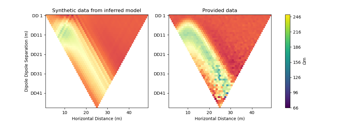
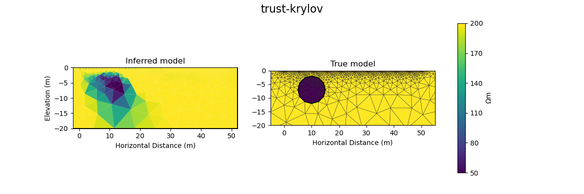
plot_result(inv_result, "trust-krylov")
Iteration #1
  objective value: 157.50708172346913
Iteration #2
  model change: 1.9999999999999998
  objective value: 68.94013122104866
Iteration #3
  model change: 2.0885981986782407
  objective value: 51.74447637863987
Iteration #4
  model change: 2.235768382076468
  objective value: 32.60775764541812
Iteration #5
  model change: 1.7295706120906689
  objective value: 29.2131751851193

Number of objective function evaluations: 6
Number of gradient function evaluations: 6
Number of hessian function evaluations: 17
Second challenge#
Iterative non linear optimisers can get trapped in a local minima, particularly if there is noise present in the data or the forward problem. The basic idea around momentum based solvers is that they account for the history of the parameter updates similarly to a ball rolling down a hill gaining momentum. They do this by computing a weighted average over past gradients. https://optimization.cbe.cornell.edu/index.php?title=Momentum
The ADAM optimiser and it variants implement such a momentum approach and are frequently used in deep learning applications, for example to train a deep neural network. https://optimization.cbe.cornell.edu/index.php?title=Adam
Here we will use the RAdam solver provided by pytorch and seek to find an optimal choice for the learning rate https://pytorch.org/docs/stable/generated/torch.optim.RAdam.html
Try to use ``RAdam`` from ``torch.optim`` and time permitting see if you can find a better value for the learning rate ``lr=`` which plays a similar role as the step length.
You may start from this template:
inv_options_torch = InversionOptions()
inv_options_torch.set_tool("CHANGE ME")
inv_options_torch.set_params(algorithm="CHANGE ME", lr=0.025, num_iterations=10, verbose=True)

inv = Inversion(ert_problem, inv_options_torch)
inv_result = inv.run()
# inv_result.summary()
print(f"\nNumber of objective function evaluations: {inv_result.n_obj_evaluations}")
print(f"Number of gradient function evaluations: {inv_result.n_grad_evaluations}")

plot_result(inv_result, "CHANGE ME")
# Copy the template above, Replace <CHANGE ME> with your answer
#@title Solution: torch.optim 'RAdam'
inv_options_torch = InversionOptions()
inv_options_torch.set_tool("torch.optim")
inv_options_torch.set_params(algorithm="RAdam", lr=0.025, num_iterations=10, verbose=True)

inv = Inversion(ert_problem, inv_options_torch)
inv_result = inv.run()
# inv_result.summary()
print(f"\nNumber of objective function evaluations: {inv_result.n_obj_evaluations}")
print(f"Number of gradient function evaluations: {inv_result.n_grad_evaluations}")

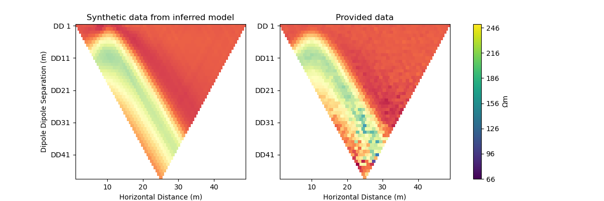
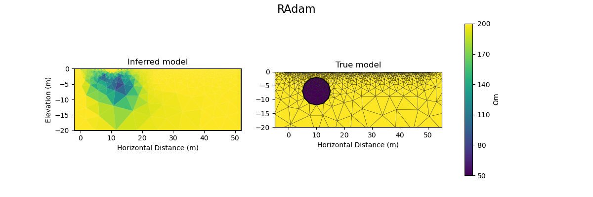
plot_result(inv_result, "RAdam")
Iteration #0, objective value: 229.71418345444994
Iteration #1, objective value: 156.9046492247734
Iteration #2, objective value: 107.12950312046189
Iteration #3, objective value: 76.24719314426017
Iteration #4, objective value: 59.9309601428337
Iteration #5, objective value: 53.93390880663932
Iteration #6, objective value: 53.88443707299642
Iteration #7, objective value: 53.813316502736185
Iteration #8, objective value: 53.72275180400689
Iteration #9, objective value: 53.615023896323265

Number of objective function evaluations: 10
Number of gradient function evaluations: 10
A word about convergence criteria…#
We have run each solver for a predetermined number of iterations and the rate at which the value of the objective function decreased was different for the different solvers. Typically, iterative non-linear algorithms terminate their iterations when a predefined fit to the data, minimum update to the model or minimum increase in fit to the data is achieved between subsequent iterations.
Where to next?#
Induced polarisation example with a real dataset! - link to notebook
Watermark#
watermark_list = ["cofi", "numpy", "scipy", "pygimli", "torch", "matplotlib"]
for pkg in watermark_list:
    pkg_var = __import__(pkg)
    print(pkg, getattr(pkg_var, "__version__"))
cofi 0.2.7
numpy 1.24.4
scipy 1.12.0
pygimli 1.4.6
torch 2.1.2.post101
matplotlib 3.8.3
sphinx_gallery_thumbnail_number = -1
Total running time of the script: (1 minutes 2.366 seconds)


