Xray Tomography

If you are running this notebook locally, make sure you’ve followed steps here to set up the environment. (This environment.yml file specifies a list of packages required to run the notebooks)

Adapted from notebooks by Andrew Valentine & Malcolm Sambridge - Research School of Earth Sciences, The Australian National University

In this notebook, we look at an linear inverse problem based on Xray Tomography. We will use cofi to run a linear system solver (optionally with Tikhonov regularization and noise estimation) for this problem.

0. Import modules

The package geo-espresso contains the forward code for this problem.

# -------------------------------------------------------- #
#                                                          #
#     Uncomment below to set up environment on "colab"     #
#                                                          #
# -------------------------------------------------------- #

# !pip install -U cofi geo-espresso
# !git clone https://github.com/inlab-geo/cofi-examples.git
# %cd cofi-examples/examples/xray_tomography

import numpy as np
from cofi import BaseProblem, InversionOptions, Inversion
from cofi.utils import QuadraticReg
from espresso import XrayTomography

1. Define the problem

# display theory on the inference problem
from IPython.display import display, Markdown

with open("../../theory/geo_xray_tomography.md", "r") as f:
    content = f.read()

display(Markdown(content))

<IPython.core.display.Markdown object>

Firstly, we get some information from the geo-espresso module. These include the dataset and the Jacobian matrix. In the Xray Tomography example, the Jacobian matrix is related to the lengths of paths within each grid. Since the paths are fixed, the Jacobian matrix stays constant.

xrt = XrayTomography()

xrt_problem = BaseProblem()
xrt_problem.set_data(xrt.data)
xrt_problem.set_jacobian(xrt.jacobian(xrt.starting_model))

Evaluating paths:   0%|          | 0/10416 [00:00<?, ?it/s]
Evaluating paths:   8%|▊         | 834/10416 [00:00<00:01, 8328.81it/s]
Evaluating paths:  16%|█▌        | 1692/10416 [00:00<00:01, 8469.66it/s]
Evaluating paths:  24%|██▍       | 2539/10416 [00:00<00:00, 8431.87it/s]
Evaluating paths:  32%|███▏      | 3383/10416 [00:00<00:00, 8413.22it/s]
Evaluating paths:  41%|████      | 4231/10416 [00:00<00:00, 8433.66it/s]
Evaluating paths:  49%|████▊     | 5075/10416 [00:00<00:00, 8425.36it/s]
Evaluating paths:  57%|█████▋    | 5926/10416 [00:00<00:00, 8450.00it/s]
Evaluating paths:  65%|██████▌   | 6789/10416 [00:00<00:00, 8505.75it/s]
Evaluating paths:  73%|███████▎  | 7640/10416 [00:00<00:00, 8415.00it/s]
Evaluating paths:  81%|████████▏ | 8489/10416 [00:01<00:00, 8437.50it/s]
Evaluating paths:  90%|████████▉ | 9346/10416 [00:01<00:00, 8476.52it/s]
Evaluating paths:  98%|█████████▊| 10198/10416 [00:01<00:00, 8488.91it/s]
Evaluating paths: 100%|██████████| 10416/10416 [00:01<00:00, 8468.34it/s]

We do some estimation on data noise and further perform a regularization.

sigma = 0.002
lamda = 50
data_cov_inv = np.identity(xrt.data_size) * (1/sigma**2)

xrt_problem.set_data_covariance_inv(data_cov_inv)
xrt_problem.set_regularization(lamda * QuadraticReg(model_shape=(xrt.model_size,)))

Review what information is included in the BaseProblem object:

xrt_problem.summary()

=====================================================================
Summary for inversion problem: BaseProblem
=====================================================================
Model shape: Unknown
---------------------------------------------------------------------
List of functions/properties set by you:
['jacobian', 'regularization', 'data', 'data_covariance_inv']
---------------------------------------------------------------------
List of functions/properties created based on what you have provided:
['jacobian_times_vector']
---------------------------------------------------------------------
List of functions/properties that can be further set for the problem:
( not all of these may be relevant to your inversion workflow )
['objective', 'log_posterior', 'log_posterior_with_blobs', 'log_likelihood', 'log_prior', 'gradient', 'hessian', 'hessian_times_vector', 'residual', 'jacobian_times_vector', 'data_misfit', 'regularization_matrix', 'forward', 'data_covariance', 'initial_model', 'model_shape', 'blobs_dtype', 'bounds', 'constraints']

2. Define the inversion options

my_options = InversionOptions()
my_options.set_tool("scipy.linalg.lstsq")

Review what’s been defined for the inversion we are about to run:

my_options.summary()

=============================
Summary for inversion options
=============================
Solving method: None set
Use `suggest_solving_methods()` to check available solving methods.
-----------------------------
Backend tool: `<class 'cofi.tools._scipy_lstsq.ScipyLstSq'>` - SciPy's wrapper function over LAPACK's linear least-squares solver, using 'gelsd', 'gelsy' (default), or 'gelss' as backend driver
References: ['https://docs.scipy.org/doc/scipy/reference/generated/scipy.linalg.lstsq.html', 'https://www.netlib.org/lapack/lug/node27.html']
Use `suggest_tools()` to check available backend tools.
-----------------------------
Solver-specific parameters: None set
Use `suggest_solver_params()` to check required/optional solver-specific parameters.

3. Start an inversion

We can now solve the inverse problem using the Tikhonov-regularized form of least-squares,

\[\mathbf{m}=\left(\mathbf{A^TA}+\epsilon^2\sigma^2\mathbf{I}\right)^\mathbf{-1}\mathbf{A^Td}\]

where \(\sigma^2\) is the variance of the expected noise on the attenuation data.

For this dataset, we’ve taken \(\sigma = 0.002\)s and chosen \(\epsilon^2 = 50\).

inv = Inversion(xrt_problem, my_options)
inv_result = inv.run()
inv_result.summary()

============================
Summary for inversion result
============================
SUCCESS
----------------------------
model: [0.98494811 1.03000048 0.95776419 ... 0.94168322 1.03668701 1.00048943]
sum_of_squared_residuals: []
effective_rank: 2500
singular_values: [9.30139732e+05 8.57631566e+05 8.57631566e+05 ... 1.14515274e+03
 8.80600410e+02 8.80600410e+02]
model_covariance: [[ 1.17571588e-04 -8.57198189e-05 -1.62727362e-06 ...  1.56635037e-07
  -6.08653282e-08 -1.36217397e-07]
 [-8.57198189e-05  2.14596891e-04 -5.56362665e-05 ... -6.06195208e-07
   4.87748993e-07 -6.08653282e-08]
 [-1.62727362e-06 -5.56362665e-05  1.35540260e-04 ...  5.04358068e-07
  -6.06195208e-07  1.56635037e-07]
 ...
 [ 1.56635037e-07 -6.06195208e-07  5.04358068e-07 ...  1.35540260e-04
  -5.56362665e-05 -1.62727362e-06]
 [-6.08653282e-08  4.87748993e-07 -6.06195208e-07 ... -5.56362665e-05
   2.14596891e-04 -8.57198189e-05]
 [-1.36217397e-07 -6.08653282e-08  1.56635037e-07 ... -1.62727362e-06
  -8.57198189e-05  1.17571588e-04]]

4. Plotting

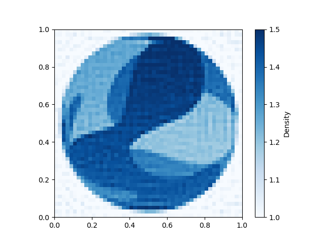
Below the two figures refers to the inferred model and true model respectively.

xrt.plot_model(inv_result.model, clim=(1, 1.5));       # inferred model
xrt.plot_model(xrt.good_model, clim=(1, 1.5));          # true model

• 
• 

<Axes: >

5. Estimated uncertainties

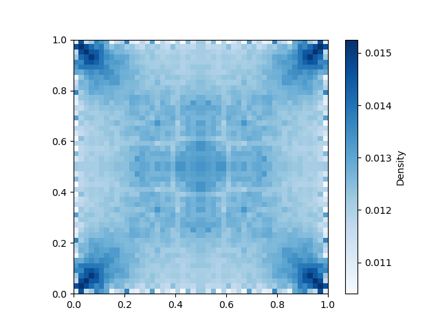
We can now find the uncertainty on the recovered slowness parameters, which describes how noise in the data propagate into the slowness parameters with this data set. For the Tikhonov-regularised form of least-squares, the model covariance matrix is a square matrix of size \(M\times M\), where there are \(M\) cells in the model.

\[\mathbf{C_m}=\sigma^2\left(\mathbf{A^TA}+\epsilon^2\sigma^2\mathbf{I}\right)^\mathbf{-1}\]

.

This matrix was calculated as part of the solver routine above. The square roots of the diagonal entries of this matrix are the \(\sigma\) errors in the slowness in each cell.

Cm = inv_result.model_covariance

Lets plot the slowness uncertainties as a function of position across the cellular model.

xrt.plot_model(np.sqrt(np.diag(Cm)));

<Axes: >

Uncertainty is uniformly low across the entire model and only significant near the corners where there are few ray paths.

Similarly we can calculate uncertainty in velocity parameters using some calculus.

\[\Delta v = \left | \frac{\partial s}{\partial v} \right | \Delta s\]

and since \(s = 1/v\) we get

\[\Delta v = s^2\Delta s\]

which gives the uncertainty image on velocity, which looks very similar.

xrt.plot_model(np.sqrt(np.diag(Cm)) * inv_result.model);

<Axes: >

By clipping the colour range you can see an imprint of the true image, indicating that high slowness/low velcoity areas have slightly higher uncertainty.

---

Watermark

watermark_list = ["cofi", "espresso", "numpy", "scipy", "matplotlib"]
for pkg in watermark_list:
    pkg_var = __import__(pkg)
    print(pkg, getattr(pkg_var, "__version__"))

cofi 0.2.7
espresso 0.3.13
numpy 1.24.4
scipy 1.12.0
matplotlib 3.8.3

sphinx_gallery_thumbnail_number = -1