Electrical Resistivity Tomography with PyGIMLi

Using the ERT (Electrical Resistivity Tomography) solver implemented provided by PyGIMLi, we use different cofi solvers to solve the corresponding inverse problem.

If you are running this notebook locally, make sure you’ve followed steps here to set up the environment. (This environment.yml file specifies a list of packages required to run the notebooks)

Note: This notebook is adapted from a PyGIMLi example: Naive complex-valued electrical inversion

0. Import modules

# -------------------------------------------------------- #
#                                                          #
#     Uncomment below to set up environment on "colab"     #
#                                                          #
# -------------------------------------------------------- #

# !pip install -U cofi

# !pip install -q condacolab
# import condacolab
# condacolab.install()
# !mamba install -c gimli pygimli=1.3

# !git clone https://github.com/inlab-geo/cofi-examples.git
# %cd cofi-examples/examples/pygimli_ert

We will need the following packages:

• numpy for matrices and matrix-related functions

• matplotlib for plotting

• pygimli for forward modelling of the problem

• cofi for accessing different inference solvers

Additionally, we wrap some pygimli code in file pygimli_ert_lib.py and import it here for conciseness.

import numpy as np
import matplotlib.pyplot as plt
import pygimli
from pygimli.physics import ert

from cofi import BaseProblem, InversionOptions, Inversion
from cofi.tools import BaseInferenceTool

from pygimli_ert_lib import *

np.random.seed(42)

1. Define the problem

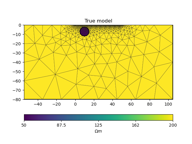
We first define the true model, the survey and map it on a computational mesh designed for the survey and true anomaly.

# PyGIMLi - define measuring scheme, geometry, forward mesh and true model
scheme = survey_scheme()
mesh, rhomap = model_true(scheme)

# plot the true model
ax = pygimli.show(mesh, data=rhomap, label="$\Omega m$", showMesh=True)
ax[0].set_title("True model")

Text(0.5, 1.0, 'True model')

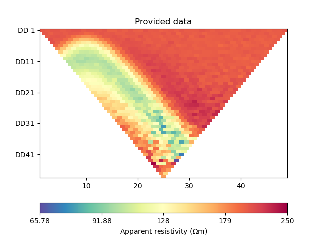
Generate the synthetic data as a container with all the necessary information for plotting.

In ERT problems, the model and data are by convention treated in log space.

# PyGIMLi - generate data
data, log_data, data_cov_inv = ert_simulate(mesh, scheme, rhomap)

ax = ert.show(data)
ax[0].set_title("Provided data")

relativeError set to a value > 0.5 .. assuming this is a percentage Error level dividing them by 100
17/04/24 - 16:47:52 - pyGIMLi - INFO - Data error estimate (min:max)  0.01000922975985971 : 0.22678548917843905

Text(0.5, 1.0, 'Provided data')

Further, we create a pygimli.ert.ERTManager instance to keep record of problem-specific information like the inversion mesh, and to perform forward operation for the inversion solvers.

# create PyGIMLi's ERT manager
ert_manager = ert_manager(data)

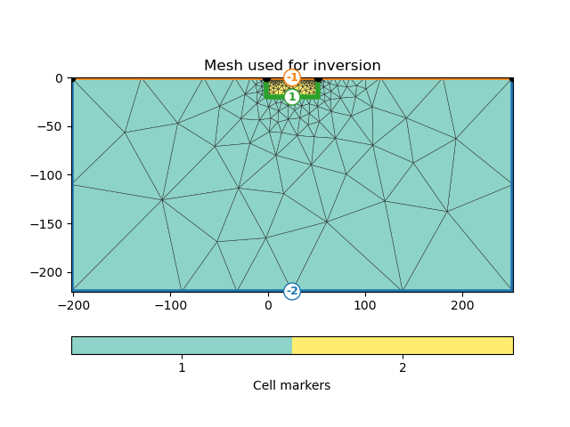
The inversion can use a different mesh and the mesh to be used should know nothing about the mesh that was designed based on the true model. We wrap two kinds of mesh as examples in the library code pygimli_ert_lib.py, namely triangular and rectangular mesh.

Use imesh_tri = inversion_mesh(scheme) to initialise a triangular mesh. This function uses PyGIMLi’s own mesh generator and generates triangular mesh automatically from given sensor locations. The resulting mesh will have a smaller area as unknowns to be inverted, as well as a background part with values prolongated outside from the parametric domain by PyGIMLi. You will see an example plot in the code cell below.

Use imesh_rect = inversion_mesh_rect(ert_manager) to initislise a rectangular mesh. The grid mesh is created from these x and y nodes: x = np.linspace(start=-5, stop=55, num=61), and y = np.linspace(start=-20,stop=0,num=10). And again, there’s a triangular background with values prolongated outside from the parametric domain by PyGIMLi.

Here we first demonstrate how to use a triangular mesh. Note that this makes the inversion problem under-determined.

inv_mesh = inversion_mesh(ert_manager)
ax = pygimli.show(inv_mesh, showMesh=True, markers=True)
ax[0].set_title("Mesh used for inversion")

17/04/24 - 16:47:53 - pyGIMLi - INFO - Found 2 regions.
17/04/24 - 16:47:53 - pyGIMLi - INFO - (ERTModelling) Region with smallest marker (1) set to background.
17/04/24 - 16:47:53 - pyGIMLi - INFO - Found 2 regions.
17/04/24 - 16:47:53 - pyGIMLi - INFO - (ERTModelling) Region with smallest marker (1) set to background.

Text(0.5, 1.0, 'Mesh used for inversion')

This folder contains examples scripts that run inversion for triangular or rectangular meshes, with different inversion approaches.

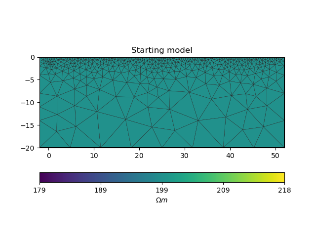
With the inversion mesh created, we now define a starting model, forward operator and weighting matrix for regularization using PyGIMLi.

Recall that both our model and data will be in log space when we perform inversion.

# PyGIMLi's forward operator (ERTModelling)
forward_oprt = ert_forward_operator(ert_manager, scheme, inv_mesh)

# extract regularization matrix
Wm = reg_matrix(forward_oprt)

# initialise a starting model for inversion
start_model, start_model_log = starting_model(ert_manager)
ax = pygimli.show(ert_manager.paraDomain, data=start_model, label="$\Omega m$", showMesh=True)
ax[0].set_title("Starting model")

17/04/24 - 16:47:53 - pyGIMLi - INFO - Creating forward mesh from region infos.
17/04/24 - 16:47:53 - pyGIMLi - INFO - Creating refined mesh (H2) to solve forward task.
17/04/24 - 16:47:53 - pyGIMLi - INFO - Mesh for forward task: Mesh: Nodes: 2198 Cells: 4124 Boundaries: 3228

Text(0.5, 1.0, 'Starting model')

CoFI and other inference packages require a set of functions that provide the misfit, the jacobian the residual within the case of scipy standardised interfaces. All these functions are defined in the library file pygimli_ert_lib.py, so open this file if you’d like to find out the details. These functions are:

• get_response

• get_jacobian

• get_residuals

• get_data_misfit

• get_regularization

• get_gradient

• get_hessian

With all the above forward operations set up with PyGIMLi, we now define the problem in cofi by setting the problem information for a BaseProblem object.

# hyperparameters
lamda = 0.0001

# CoFI - define BaseProblem
ert_problem = BaseProblem()
ert_problem.name = "Electrical Resistivity Tomography defined through PyGIMLi"
ert_problem.set_forward(get_response, args=[forward_oprt])
ert_problem.set_jacobian(get_jacobian, args=[forward_oprt])
ert_problem.set_residual(get_residual, args=[log_data, forward_oprt])
ert_problem.set_data_misfit(get_data_misfit, args=[log_data, forward_oprt, data_cov_inv])
ert_problem.set_regularization(get_regularization, args=[Wm, lamda])
ert_problem.set_gradient(get_gradient, args=[log_data, forward_oprt, Wm, lamda, data_cov_inv])
ert_problem.set_hessian(get_hessian, args=[log_data, forward_oprt, Wm, lamda, data_cov_inv])
ert_problem.set_initial_model(start_model_log)

Review what information is included in the BaseProblem object:

ert_problem.summary()

========================================================================================
Summary for inversion problem: Electrical Resistivity Tomography defined through PyGIMLi
========================================================================================
Model shape: (831,)
----------------------------------------------------------------------------------------
List of functions/properties set by you:
['gradient', 'hessian', 'residual', 'jacobian', 'data_misfit', 'regularization', 'forward', 'initial_model', 'model_shape']
----------------------------------------------------------------------------------------
List of functions/properties created based on what you have provided:
['objective', 'hessian_times_vector', 'jacobian_times_vector']
----------------------------------------------------------------------------------------
List of functions/properties that can be further set for the problem:
( not all of these may be relevant to your inversion workflow )
['objective', 'log_posterior', 'log_posterior_with_blobs', 'log_likelihood', 'log_prior', 'hessian_times_vector', 'jacobian_times_vector', 'regularization_matrix', 'data', 'data_covariance', 'data_covariance_inv', 'blobs_dtype', 'bounds', 'constraints']

2. Define the inversion options and run

SciPy’s optimizer (trust-exact)

ert_problem.suggest_tools();

Based on what you've provided so far, here are possible tools:
{
    "optimization": [
        "scipy.optimize.minimize",
        "scipy.optimize.least_squares",
        "torch.optim"
    ],
    "matrix solvers": [
        "cofi.simple_newton"
    ],
    "sampling": [
        "bayesbay",
        "neighpy"
    ]
}

{'optimization': ['scipy.optimize.minimize', 'scipy.optimize.least_squares', 'torch.optim'], 'matrix solvers': ['cofi.simple_newton'], 'sampling': ['bayesbay', 'neighpy']}

inv_options_scipy = InversionOptions()
inv_options_scipy.set_tool("scipy.optimize.minimize")
inv_options_scipy.set_params(method="trust-exact", options={"maxiter": 10})

Review what’s been defined for the inversion we are about to run:

inv_options_scipy.summary()

=============================
Summary for inversion options
=============================
Solving method: None set
Use `suggest_solving_methods()` to check available solving methods.
-----------------------------
Backend tool: `<class 'cofi.tools._scipy_opt_min.ScipyOptMin'>` - SciPy's optimizers that minimizes a scalar function with respect to one or more variables, check SciPy's documentation page for a list of methods
References: ['https://docs.scipy.org/doc/scipy/reference/generated/scipy.optimize.minimize.html']
Use `suggest_tools()` to check available backend tools.
-----------------------------
Solver-specific parameters:
method = trust-exact
options = {'maxiter': 10}
Use `suggest_solver_params()` to check required/optional solver-specific parameters.

inv = Inversion(ert_problem, inv_options_scipy)
inv_result = inv.run()
# inv_result.summary()
print(f"\nSolver message: {inv_result.message}")

/home/jiawen/opt/mambaforge/envs/cofi_dev/lib/python3.10/site-packages/cofi/tools/_scipy_opt_min.py:103: RuntimeWarning: Method trust-exact does not use Hessian-vector product information (hessp).
  return minimize(

Solver message: Maximum number of iterations has been exceeded.

inv_result.success

False

Plot the results:

# convert back to normal space from log space
model = np.exp(inv_result.model)

# plot inferred model
ax = pygimli.show(ert_manager.paraDomain, data=model, label=r"$\Omega m$")
ax[0].set_title("Inferred model")

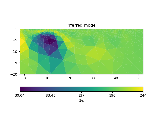
Text(0.5, 1.0, 'Inferred model')

We can now also compare the synthetic data with provided observations.

_, axes = plt.subplots(1, 2, figsize=(12,4))

# plot synthetic data
d = forward_oprt.response(model)
ert.showERTData(scheme, vals=d, cMin=np.min(data["rhoa"]), cMax=np.max(data["rhoa"]), ax=axes[0])
axes[0].set_title("Synthetic data from inferred model")

# plot given data
ert.show(data, ax=axes[1])
axes[1].set_title("Provided data")

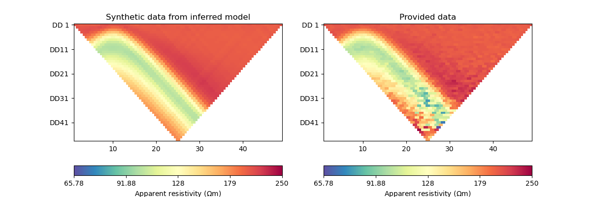
Text(0.5, 1.0, 'Provided data')

3. What’s next?

Now that we’ve seen the PyGIMLi ERT problem solved by two different inversion approaches through CoFI, it would be nice to see more inversion solvers (even a sampler!) and a similar problem defined with a rectangular mesh. If you’d like to see some self-contained examples, head to this GitHub folder to explore more.

---

Watermark

watermark_list = ["cofi", "numpy", "scipy", "pygimli", "matplotlib"]
for pkg in watermark_list:
    pkg_var = __import__(pkg)
    print(pkg, getattr(pkg_var, "__version__"))

cofi 0.2.7
numpy 1.24.4
scipy 1.12.0
pygimli 1.5.0
matplotlib 3.8.3

sphinx_gallery_thumbnail_number = -1