
Note
Go to the end to download the full example code.
1D Rayleigh wave phase velocity inversion#
If you are running this notebook locally, make sure you’ve followed steps here to set up the environment. (This environment.yml file specifies a list of packages required to run the notebooks)
What we do in this notebook#
Here we look at applying CoFI to the inversion of Rayleigh wave phase velocities for a 1D layered earth.
Learning outcomes
A demonstration of CoFI’s ability to switch between parameter estimation and ensemble methods.
A comparison between different McMC samplers that is fixed-d and trans-d samplers
An application of CoFI to field data
# -------------------------------------------------------- #
#                                                          #
#     Uncomment below to set up environment on "colab"     #
#                                                          #
# -------------------------------------------------------- #

# !pip install -U cofi git+https://github.com/inlab-geo/pysurf96.git
# !git clone https://github.com/inlab-geo/cofi-examples.git
# %cd cofi-examples/tutorials/rayleigh_wave_phase_velocity
# If this notebook is run locally pysurf96 needs to be installed separately by uncommenting the following line,
# that is by removing the # and the white space between it and the exclamation mark.
# !pip install -U cofi git+https://github.com/inlab-geo/pysurf96.git
import numpy as np
import scipy
import matplotlib.pyplot as plt

from pysurf96 import surf96
import bayesbay
import cofi
Problem description#
Here we illustrate the range of inversion methods made avaialbe by CoFI. That is we first define a base problem and then explore the use of an iterative non linear apporach to find the MAP solution and then employ a range of Markov Chain Monte Carlo strategies to recover the posterior distribution. The forward problem is solved using pysurf 96 (miili/pysurf96) and the field data example is taken from (https://www.eas.slu.edu/eqc/eqc_cps/TUTORIAL/STRUCT/index.html) and we will be inverting observed rayleigh wave phase velocities
Inference problem
# display theory on the inference problem
from IPython.display import display, Markdown

with open("../../theory/geo_surface_wave_dispersion.md", "r") as f:
    content = f.read()

display(Markdown(content))
<IPython.core.display.Markdown object>
Solving methods
# display theory on the optimisation approach
with open("../../theory/inv_optimisation.md", "r") as f:
    content = f.read()

display(Markdown(content))
<IPython.core.display.Markdown object>
# display theory on the optimisation approach
with open("../../theory/inv_mcmc.md", "r") as f:
    content = f.read()

display(Markdown(content))
<IPython.core.display.Markdown object>
Further reading
Utilities#
1D model paramterisation#
# display theory on the 1D model parameterisation
with open("../../theory/misc_1d_model_parameterisation.md", "r") as f:
    content = f.read()

display(Markdown(content))
<IPython.core.display.Markdown object>
# layercake model utilities
def form_layercake_model(thicknesses, vs):
    model = np.zeros((len(vs)*2-1,))
    model[1::2] = thicknesses
    model[::2] = vs
    return model

def split_layercake_model(model):
    thicknesses = model[1::2]
    vs = model[::2]
    return thicknesses, vs
# voronoi model utilities
def form_voronoi_model(voronoi_sites, vs):
    return np.hstack((vs, voronoi_sites))

def split_voronoi_model(model):
    voronoi_sites = model[len(model)//2:]
    vs = model[:len(model)//2]
    return voronoi_sites, vs
def voronoi_to_layercake(voronoi_vector: np.ndarray) -> np.ndarray:
    n_layers = len(voronoi_vector) // 2
    velocities = voronoi_vector[:n_layers]
    voronoi_sites = voronoi_vector[n_layers:]
    depths = (voronoi_sites[:-1] + voronoi_sites[1:]) / 2
    thicknesses = depths - np.insert(depths[:-1], 0, 0)
    layercake_vector = np.zeros((2*n_layers-1,))
    layercake_vector[::2] = velocities
    layercake_vector[1::2] = thicknesses
    return layercake_vector

def layercake_to_voronoi(layercake_vector: np.ndarray, first_voronoi_site: float = 0.0) -> np.ndarray:
    n_layers = len(layercake_vector) // 2 + 1
    thicknesses = layercake_vector[1::2]
    velocities = layercake_vector[::2]
    depths = np.cumsum(thicknesses)
    voronoi_sites = np.zeros((n_layers,))
    for i in range(1,len(voronoi_sites)):
        voronoi_sites[i] = 2 * depths[i-1] - voronoi_sites[i-1]
    voronoi_vector = np.hstack((velocities, voronoi_sites))
    return voronoi_vector
Forward solver#
# display theory on the using the forward solver
with open("../../theory/geo_surface_wave_dispersion2.md", "r") as f:
    content = f.read()

display(Markdown(content))
<IPython.core.display.Markdown object>
# Constants
VP_VS = 1.77
RHO_VP_K = 0.32
RHO_VP_B = 0.77
# forward through pysurf96
def forward_sw(model, periods):
    thicknesses, vs = split_layercake_model(model)
    thicknesses = np.append(thicknesses, 10)
    vp = vs * VP_VS
    rho = RHO_VP_K * vp + RHO_VP_B
    return surf96(
        thicknesses,
        vp,
        vs,
        rho,
        periods,
        wave="rayleigh",
        mode=1,
        velocity="phase",
        flat_earth=False,
    )

# numerical jacobian
def jacobian_sw(model, periods, fwd=forward_sw, relative_step=0.01):
    jacobian = np.zeros((len(periods), len(model)))
    original_dpred = fwd(model, periods)
    for i in range(len(model)):
        perturbed_model = model.copy()
        step = relative_step * model[i]
        perturbed_model[i] += step
        perturbed_dpred = fwd(perturbed_model, periods)
        derivative = (perturbed_dpred - original_dpred) / abs(step)
        jacobian[:, i] = derivative
    return jacobian
Visualisation#
For conveninece we also implement two functions to plot the data here the Rayleigh wave phase velocity and a model given in the layer based parametrisation.
def plot_model(model, ax=None, title="model", **kwargs):
    # process data
    thicknesses = np.append(model[1::2], max(model[1::2]))
    velocities = model[::2]
    y = np.insert(np.cumsum(thicknesses), 0, 0)
    x = np.insert(velocities, 0, velocities[0])

    # plot depth profile
    if ax is None:
        _, ax = plt.subplots()
    plotting_style = {
        "linewidth": kwargs.pop("linewidth", kwargs.pop("lw", 0.5)),
        "alpha": 0.2,
        "color": kwargs.pop("color", kwargs.pop("c", "blue")),
    }
    plotting_style.update(kwargs)
    ax.step(x, y, where="post", **plotting_style)
    if ax.get_ylim()[0] < ax.get_ylim()[1]:
        ax.invert_yaxis()
    ax.set_xlabel("Vs (km/s)")
    ax.set_ylabel("Depth (km)")
    ax.set_title(title)
    return ax
def plot_data(rayleigh_phase_velocities, periods, ax=None, scatter=False,
              title="data", **kwargs):
    if ax is None:
        _, ax = plt.subplots()
    plotting_style = {
        "linewidth": kwargs.pop("linewidth", kwargs.pop("lw", 1)),
        "alpha": 1,
        "color": kwargs.pop("color", kwargs.pop("c", "blue")),
    }
    plotting_style.update(**kwargs)
    if scatter:
        ax.scatter(periods, rayleigh_phase_velocities, **plotting_style)
    else:
        ax.plot(periods, rayleigh_phase_velocities, **plotting_style)
    ax.set_xlabel("Periods (s)")
    ax.set_ylabel("Rayleigh phase velocities (km/s)")
    ax.set_title(title)
    return ax
def plot_model_and_data(model, label_model, color_model,
                        forward_func, periods, label_d_pred, color_d_pred,
                        axes=None, light_thin=False):
    if axes is None:
        _, axes = plt.subplots(1, 2, figsize=(10, 4), gridspec_kw={"width_ratios": [1, 2.5]})
    ax1, ax2 = axes
    if light_thin:
        plot_model(model, ax=ax1, color=color_model, alpha=0.2, lw=0.5, label=label_model)
        plot_data(forward_func(model, periods), periods, ax=ax2, color=color_d_pred, alpha=0.2, lw=0.5, label=label_d_pred)
    else:
        plot_model(model, ax=ax1, color=color_model, alpha=1, lw=1, label=label_model)
        plot_data(forward_func(model, periods), periods, ax=ax2, color=color_d_pred, label=label_d_pred)
    ax1.legend()
    ax2.legend()
    return ax1, ax2
Synthetic example#
Prior to inverting any field data it is good practice to test an inversion method using sythetic exmaples where we know the true model. It is also recommended to prior to this idnepently test any forward solver that is being used and verify the Jacobian, as problems related to the forward sovler are diffiuclt to identify and diagnose once they are integrated in an inversion methodology.
Generate synthetic data#
synth_d_periods = np.geomspace(3, 80, 20)

true_thicknesses = np.array([10, 10, 15, 20, 20, 20, 20, 20])
true_vs = np.array([3.38, 3.44, 3.66, 4.25, 4.35, 4.32, 4.315, 4.38, 4.5])
true_model = form_layercake_model(true_thicknesses, true_vs)
noise_level = 0.02
d_true = forward_sw(true_model, synth_d_periods)
d_obs = d_true + np.random.normal(0, 0.01, len(d_true))
# plot true model and d_pred from true model
_, ax2 = plot_model_and_data(model=true_model, label_model="true model", color_model="orange",
                    forward_func=forward_sw, periods=synth_d_periods,
                    label_d_pred="true data (noiseless)", color_d_pred="orange")

# plot d_obs
plot_data(d_obs, synth_d_periods, ax=ax2, scatter=True, color="red", s=20, label="observed data (noisy)")
ax2.legend();
<matplotlib.legend.Legend object at 0x7efdb46c6fd0>
Optimisation#
Prepare ``BaseProblem`` for optimisation
n_dims = 17

init_thicknesses = np.ones((n_dims//2,)) * 15
init_vs = np.ones((n_dims//2+1,)) * 4.0
init_model = form_layercake_model(init_thicknesses, init_vs)
# plot the model and d_pred for starting model
axes = plot_model_and_data(model=init_model, label_model="starting model", color_model="purple",
                           forward_func=forward_sw, periods=synth_d_periods,
                           label_d_pred="data predictions from starting model", color_d_pred="purple")

# plot the model and d_pred for true model
plot_model_and_data(model=true_model, label_model="true model", color_model="orange",
                    forward_func=forward_sw, periods=synth_d_periods,
                    label_d_pred="true data (noiseless)", color_d_pred="orange", axes=axes)

# plot d_obs
plot_data(d_obs, synth_d_periods, ax=axes[1], scatter=True, color="red", s=20, label="d_obs")
axes[1].legend();
<matplotlib.legend.Legend object at 0x7efd941f3ed0>
my_reg = cofi.utils.QuadraticReg(
    weighting_matrix="damping",
    model_shape=(n_dims,),
    reference_model=init_model
)
def my_objective(model, fwd, periods, d_obs, lamda=1.0):
    d_pred = fwd(model, periods)
    data_misfit = np.sum((d_obs - d_pred) ** 2)
    reg = my_reg(model)
    return data_misfit + lamda * reg

def my_objective_gradient(model, fwd, periods, d_obs, lamda=1.0):
    d_pred = fwd(model, periods)
    jac = jacobian_sw(model, periods, fwd)
    data_misfit_grad = -2 * jac.T @ (d_obs - d_pred)
    reg_grad = my_reg.gradient(model)
    return data_misfit_grad + lamda * reg_grad

def my_objective_hessian(model, fwd, periods, d_obs, lamda=1.0):
    jac = jacobian_sw(model, periods, fwd)
    data_misfit_hess = 2 * jac.T @ jac
    reg_hess = my_reg.hessian(model)
    return data_misfit_hess + lamda * reg_hess
Optimisation with no damping#
lamda = 0

kwargs = {
    "fwd": forward_sw,
    "periods": synth_d_periods,
    "d_obs": d_obs,
    "lamda": lamda
}
sw_problem_no_reg = cofi.BaseProblem()
sw_problem_no_reg.set_objective(my_objective, kwargs=kwargs)
sw_problem_no_reg.set_gradient(my_objective_gradient, kwargs=kwargs)
sw_problem_no_reg.set_hessian(my_objective_hessian, kwargs=kwargs)
sw_problem_no_reg.set_initial_model(init_model)
Define ``InversionOptions``
inv_options_optimiser = cofi.InversionOptions()
inv_options_optimiser.set_tool("scipy.optimize.minimize")
inv_options_optimiser.set_params(method="trust-exact")
Define ``Inversion`` and run
inv_optimiser_no_reg = cofi.Inversion(sw_problem_no_reg, inv_options_optimiser)
inv_result_optimiser_no_reg = inv_optimiser_no_reg.run()
Plot results
# plot the model and d_pred for starting model
axes = plot_model_and_data(model=init_model, label_model="starting model", color_model="black",
                           forward_func=forward_sw, periods=synth_d_periods,
                           label_d_pred="d_pred from starting model", color_d_pred="black")

# plot the model and d_pred for true model
plot_model_and_data(model=true_model, label_model="true model", color_model="orange",
                    forward_func=forward_sw, periods=synth_d_periods,
                    label_d_pred="d_pred from true model", color_d_pred="orange", axes=axes)

# plot the model and d_pred for inverted model
plot_model_and_data(model=inv_result_optimiser_no_reg.model, label_model="inverted model", color_model="purple",
                    forward_func=forward_sw, periods=synth_d_periods,
                    label_d_pred="d_pred from inverted model", color_d_pred="purple", axes=axes);

# plot d_obs
plot_data(d_obs, synth_d_periods, ax=axes[1], scatter=True, color="red", s=20, label="d_obs")
axes[1].legend();
<matplotlib.legend.Legend object at 0x7efda2416210>
Optimal damping#
Obviously we get a very skewed 1D model out of an optimisation that solely tries to minimise the data misfit. We would like to add a damping term to our objective function, but we are not sure which factor suits the problem well.
In this situation, the InversionPool from CoFI can be handy.
lambdas = np.logspace(-6, 6, 15)

my_lcurve_problems = []
for lamb in lambdas:
    my_problem = cofi.BaseProblem()
    kwargs = {
        "fwd": forward_sw,
        "periods": synth_d_periods,
        "d_obs": d_obs,
        "lamda": lamb
    }
    my_problem.set_objective(my_objective, kwargs=kwargs)
    my_problem.set_gradient(my_objective_gradient, kwargs=kwargs)
    my_problem.set_hessian(my_objective_hessian, kwargs=kwargs)
    my_problem.set_initial_model(init_model)
    my_lcurve_problems.append(my_problem)

def my_callback(inv_result, i):
    m = inv_result.model
    res_norm = np.linalg.norm(forward_sw(m, synth_d_periods) - d_obs)
    reg_norm = np.sqrt(my_reg(m))
    print(f"Finished inversion with lambda={lambdas[i]}: {res_norm}, {reg_norm}")
    return res_norm, reg_norm

my_inversion_pool = cofi.utils.InversionPool(
    list_of_inv_problems=my_lcurve_problems,
    list_of_inv_options=inv_options_optimiser,
    callback=my_callback,
    parallel=False
)
all_res, all_cb_returns = my_inversion_pool.run()

l_curve_points = list(zip(*all_cb_returns))
Finished inversion with lambda=1e-06: 0.0203050470011874, 2.4275757169615164
Finished inversion with lambda=7.196856730011514e-06: 0.020556709540535893, 1.5087454125573867
Finished inversion with lambda=5.1794746792312125e-05: 0.020842898411810147, 1.2478449878253486
Finished inversion with lambda=0.0003727593720314938: 0.021287899207720434, 1.1861328243575346
Finished inversion with lambda=0.0026826957952797246: 0.02310193636700535, 1.1554256090471304
Finished inversion with lambda=0.019306977288832496: 0.036432160801205246, 1.1194246137168853
Finished inversion with lambda=0.1389495494373136: 0.1495689268318053, 0.9824128014140784
Finished inversion with lambda=1.0: 0.5003804737348793, 0.6597634671073339
Finished inversion with lambda=7.196856730011514: 1.102762629560565, 0.3145983936600282
Finished inversion with lambda=51.79474679231202: 1.630087241402099, 0.06790929620393707
Finished inversion with lambda=372.7593720314938: 1.755519406666188, 0.010159672806182681
Finished inversion with lambda=2682.6957952797275: 1.7744804308847013, 0.0014265729685016275
Finished inversion with lambda=19306.977288832455: 1.7771486123740319, 0.00019848218327743044
Finished inversion with lambda=138949.5494373136: 1.7775253027742732, 2.7585620343800265e-05
Finished inversion with lambda=1000000.0: 1.7775763022040398, 3.833137180454159e-06
# print all the lambdas
lambdas
array([1.00000000e-06, 7.19685673e-06, 5.17947468e-05, 3.72759372e-04,
       2.68269580e-03, 1.93069773e-02, 1.38949549e-01, 1.00000000e+00,
       7.19685673e+00, 5.17947468e+01, 3.72759372e+02, 2.68269580e+03,
       1.93069773e+04, 1.38949549e+05, 1.00000000e+06])
Plot L-curve
# plot the L-curve
res_norm, reg_norm = l_curve_points
plt.plot(reg_norm, res_norm, '.-')
plt.xlabel(r'Norm of regularization term $||Wm||_2$')
plt.ylabel(r'Norm of residual $||g(m)-d||_2$')
for i in range(0, len(lambdas), 2):
    plt.annotate(f'{lambdas[i]:.1e}', (reg_norm[i], res_norm[i]), fontsize=8)
Optimisation with damping#
From the L-curve plot above, it seems that a damping factor of around 0.02 would be good.
lamda = 0.02

kwargs = {
    "fwd": forward_sw,
    "periods": synth_d_periods,
    "d_obs": d_obs,
    "lamda": lamda
}
sw_problem = cofi.BaseProblem()
sw_problem.set_objective(my_objective, kwargs=kwargs)
sw_problem.set_gradient(my_objective_gradient, kwargs=kwargs)
sw_problem.set_hessian(my_objective_hessian, kwargs=kwargs)
sw_problem.set_initial_model(init_model)
Define ``Inversion`` and run
inv_optimiser = cofi.Inversion(sw_problem, inv_options_optimiser)
inv_result_optimiser = inv_optimiser.run()
Plot results
# plot the model and d_pred for starting model
axes = plot_model_and_data(model=init_model, label_model="starting model", color_model="black",
                           forward_func=forward_sw, periods=synth_d_periods,
                           label_d_pred="d_pred from starting model", color_d_pred="black")

# plot the model and d_pred for true model
plot_model_and_data(model=true_model, label_model="true model", color_model="orange",
                    forward_func=forward_sw, periods=synth_d_periods,
                    label_d_pred="d_pred from true model", color_d_pred="orange", axes=axes)

# plot the model and d_pred for damped solution, and d_obs
plot_model_and_data(model=inv_result_optimiser.model, label_model="damped solution", color_model="purple",
                    forward_func=forward_sw, periods=synth_d_periods,
                    label_d_pred="d_pred from damped solution", color_d_pred="purple", axes=axes);

# plot d_obs
plot_data(d_obs, synth_d_periods, ax=axes[1], scatter=True, color="red", s=20, label="d_obs")
axes[1].legend();
<matplotlib.legend.Legend object at 0x7efda58c8e10>
Fixed-dimensional sampling#
Prepare ``BaseProblem`` for fixed-dimensional sampling
thick_min = 5
thick_max = 30
vs_min = 2
vs_max = 5

def my_log_prior(model):
    thicknesses, vs = split_layercake_model(model)
    thicknesses_out_of_bounds = (thicknesses < thick_min) | (thicknesses > thick_max)
    vs_out_of_bounds = (vs < vs_min) | (vs > vs_max)
    if np.any(thicknesses_out_of_bounds) or np.any(vs_out_of_bounds):
        return float("-inf")
    log_prior = -np.log(thick_max - thick_min) * len(thicknesses) - np.log(vs_max - vs_min) * len(vs)
    return log_prior
Cdinv = np.eye(len(d_obs))/(noise_level**2)      # inverse data covariance matrix

def my_log_likelihood(model):
    try:
        d_pred = forward_sw(model, synth_d_periods)
    except:
        return float("-inf")
    residual = d_obs - d_pred
    return -0.5 * residual @ (Cdinv @ residual).T
n_walkers = 40

my_walkers_start = np.ones((n_walkers, n_dims)) * inv_result_optimiser.model
for i in range(n_walkers):
    my_walkers_start[i,:] += np.random.normal(0, 0.3, n_dims)
sw_problem.set_log_prior(my_log_prior)
sw_problem.set_log_likelihood(my_log_likelihood)
Define ``InversionOptions``
inv_options_fixed_d_sampling = cofi.InversionOptions()
inv_options_fixed_d_sampling.set_tool("emcee")
inv_options_fixed_d_sampling.set_params(
    nwalkers=n_walkers,
    nsteps=2_000,
    initial_state=my_walkers_start,
    skip_initial_state_check=True,
    progress=True
)
Define ``Inversion`` and run
We will disable the display of warnings temporarily due to the
unavoidable existence of -inf in our prior.
np.seterr(all="ignore");
{'divide': 'ignore', 'over': 'ignore', 'under': 'ignore', 'invalid': 'ignore'}
Sample the prior#
prior_sampling_problem = cofi.BaseProblem()
prior_sampling_problem.set_log_posterior(my_log_prior)
prior_sampling_problem.set_model_shape(init_model.shape)
prior_sampler = cofi.Inversion(prior_sampling_problem, inv_options_fixed_d_sampling)
prior_results = prior_sampler.run()
  0%|          | 0/2000 [00:00<?, ?it/s]
  6%|▌         | 112/2000 [00:00<00:01, 1114.91it/s]
 11%|█▏        | 228/2000 [00:00<00:01, 1139.85it/s]
 17%|█▋        | 345/2000 [00:00<00:01, 1152.02it/s]
 23%|██▎       | 464/2000 [00:00<00:01, 1163.13it/s]
 29%|██▉       | 582/2000 [00:00<00:01, 1167.61it/s]
 35%|███▍      | 699/2000 [00:00<00:01, 1166.42it/s]
 41%|████      | 816/2000 [00:00<00:01, 1158.56it/s]
 47%|████▋     | 932/2000 [00:00<00:00, 1155.13it/s]
 52%|█████▎    | 1050/2000 [00:00<00:00, 1160.96it/s]
 58%|█████▊    | 1167/2000 [00:01<00:00, 1162.15it/s]
 64%|██████▍   | 1285/2000 [00:01<00:00, 1165.58it/s]
 70%|███████   | 1402/2000 [00:01<00:00, 1165.17it/s]
 76%|███████▌  | 1521/2000 [00:01<00:00, 1169.73it/s]
 82%|████████▏ | 1640/2000 [00:01<00:00, 1173.19it/s]
 88%|████████▊ | 1759/2000 [00:01<00:00, 1175.94it/s]
 94%|█████████▍| 1877/2000 [00:01<00:00, 1176.18it/s]
100%|█████████▉| 1996/2000 [00:01<00:00, 1179.50it/s]
100%|██████████| 2000/2000 [00:01<00:00, 1166.54it/s]
import arviz as az

labels = ["v0", "t0", "v1", "t1", "v2", "t2", "v3", "t3", "v4", "t4", "v5", "t5", "v6", "t6", "v7", "t7", "v8"]

prior_results_sampler = prior_results.sampler
az_idata_prior = az.from_emcee(prior_results_sampler, var_names=labels)

pc = az.plot_trace_dist(
    az_idata_prior,
    visuals={"xlabel_trace": False, "trace": {"color": "C0"}, "dist": {"color": "C0"}},
    figure_kwargs={"figsize": (10, 25), "constrained_layout": True},
)

n_vars = len(az_idata_prior.posterior.data_vars)
var_names = list(az_idata_prior.posterior.data_vars)
for i in range(n_vars):
    ax1 = pc.iget_target(i, 0)
    ax2 = pc.iget_target(i, 1)
    ax1.set_title(var_names[i])
    ax1.set_xlabel("parameter value")
    ax1.set_ylabel("density value")
    ax2.set_title(var_names[i])
    ax2.set_xlabel("number of iterations")
    ax2.set_ylabel("parameter value")
    ax2.margins(x=0)
Sample the posterior#
inversion_fixed_d_sampler = cofi.Inversion(sw_problem, inv_options_fixed_d_sampling)
inv_result_fixed_d_sampler = inversion_fixed_d_sampler.run()
  0%|          | 0/2000 [00:00<?, ?it/s]
  0%|          | 7/2000 [00:00<00:31, 63.03it/s]
  1%|          | 14/2000 [00:00<00:32, 61.48it/s]
  1%|          | 21/2000 [00:00<00:34, 58.06it/s]
  1%|▏         | 27/2000 [00:00<00:36, 54.72it/s]
  2%|▏         | 33/2000 [00:00<00:35, 55.02it/s]
  2%|▏         | 39/2000 [00:00<00:36, 54.43it/s]
  2%|▏         | 45/2000 [00:00<00:35, 54.92it/s]
  3%|▎         | 51/2000 [00:00<00:34, 55.72it/s]
  3%|▎         | 57/2000 [00:01<00:34, 56.79it/s]
  3%|▎         | 63/2000 [00:01<00:34, 56.03it/s]
  3%|▎         | 69/2000 [00:01<00:34, 56.43it/s]
  4%|▍         | 76/2000 [00:01<00:33, 58.15it/s]
  4%|▍         | 83/2000 [00:01<00:32, 59.63it/s]
  4%|▍         | 90/2000 [00:01<00:30, 62.08it/s]
  5%|▍         | 97/2000 [00:01<00:30, 63.12it/s]
  5%|▌         | 104/2000 [00:01<00:29, 64.07it/s]
  6%|▌         | 111/2000 [00:01<00:28, 65.48it/s]
  6%|▌         | 118/2000 [00:01<00:28, 66.61it/s]
  6%|▋         | 126/2000 [00:02<00:27, 68.80it/s]
  7%|▋         | 134/2000 [00:02<00:26, 69.81it/s]
  7%|▋         | 142/2000 [00:02<00:26, 71.30it/s]
  8%|▊         | 150/2000 [00:02<00:25, 71.86it/s]
  8%|▊         | 158/2000 [00:02<00:25, 72.05it/s]
  8%|▊         | 166/2000 [00:02<00:25, 71.13it/s]
  9%|▊         | 174/2000 [00:02<00:25, 70.35it/s]
  9%|▉         | 182/2000 [00:02<00:25, 70.73it/s]
 10%|▉         | 190/2000 [00:02<00:25, 70.76it/s]
 10%|▉         | 198/2000 [00:03<00:25, 70.27it/s]
 10%|█         | 206/2000 [00:03<00:25, 70.71it/s]
 11%|█         | 214/2000 [00:03<00:24, 71.51it/s]
 11%|█         | 222/2000 [00:03<00:24, 72.95it/s]
 12%|█▏        | 231/2000 [00:03<00:23, 75.04it/s]
 12%|█▏        | 239/2000 [00:03<00:23, 75.85it/s]
 12%|█▏        | 248/2000 [00:03<00:22, 78.52it/s]
 13%|█▎        | 257/2000 [00:03<00:21, 80.94it/s]
 13%|█▎        | 266/2000 [00:03<00:21, 82.41it/s]
 14%|█▍        | 275/2000 [00:04<00:20, 83.94it/s]
 14%|█▍        | 284/2000 [00:04<00:20, 84.41it/s]
 15%|█▍        | 293/2000 [00:04<00:20, 85.30it/s]
 15%|█▌        | 302/2000 [00:04<00:19, 86.09it/s]
 16%|█▌        | 312/2000 [00:04<00:19, 88.31it/s]
 16%|█▌        | 321/2000 [00:04<00:19, 88.06it/s]
 17%|█▋        | 331/2000 [00:04<00:18, 90.89it/s]
 17%|█▋        | 341/2000 [00:04<00:18, 92.06it/s]
 18%|█▊        | 351/2000 [00:04<00:18, 91.11it/s]
 18%|█▊        | 361/2000 [00:04<00:18, 90.67it/s]
 19%|█▊        | 371/2000 [00:05<00:18, 88.68it/s]
 19%|█▉        | 381/2000 [00:05<00:17, 91.23it/s]
 20%|█▉        | 391/2000 [00:05<00:17, 90.34it/s]
 20%|██        | 401/2000 [00:05<00:17, 91.88it/s]
 21%|██        | 411/2000 [00:05<00:18, 88.14it/s]
 21%|██        | 420/2000 [00:05<00:18, 87.04it/s]
 21%|██▏       | 429/2000 [00:05<00:18, 86.32it/s]
 22%|██▏       | 439/2000 [00:05<00:17, 88.00it/s]
 22%|██▏       | 449/2000 [00:05<00:17, 89.38it/s]
 23%|██▎       | 458/2000 [00:06<00:17, 87.51it/s]
 23%|██▎       | 467/2000 [00:06<00:17, 87.48it/s]
 24%|██▍       | 476/2000 [00:06<00:17, 86.24it/s]
 24%|██▍       | 485/2000 [00:06<00:17, 85.79it/s]
 25%|██▍       | 495/2000 [00:06<00:17, 87.15it/s]
 25%|██▌       | 504/2000 [00:06<00:17, 87.87it/s]
 26%|██▌       | 513/2000 [00:06<00:17, 87.11it/s]
 26%|██▌       | 523/2000 [00:06<00:16, 88.51it/s]
 27%|██▋       | 532/2000 [00:06<00:16, 88.61it/s]
 27%|██▋       | 541/2000 [00:07<00:16, 88.92it/s]
 28%|██▊       | 550/2000 [00:07<00:16, 88.17it/s]
 28%|██▊       | 560/2000 [00:07<00:15, 90.39it/s]
 28%|██▊       | 570/2000 [00:07<00:16, 89.36it/s]
 29%|██▉       | 580/2000 [00:07<00:15, 89.87it/s]
 29%|██▉       | 589/2000 [00:07<00:16, 88.09it/s]
 30%|██▉       | 599/2000 [00:07<00:15, 90.46it/s]
 30%|███       | 609/2000 [00:07<00:15, 90.64it/s]
 31%|███       | 619/2000 [00:07<00:14, 92.72it/s]
 32%|███▏      | 630/2000 [00:08<00:14, 95.88it/s]
 32%|███▏      | 641/2000 [00:08<00:13, 97.16it/s]
 33%|███▎      | 651/2000 [00:08<00:14, 92.85it/s]
 33%|███▎      | 661/2000 [00:08<00:14, 93.94it/s]
 34%|███▎      | 671/2000 [00:08<00:14, 94.05it/s]
 34%|███▍      | 681/2000 [00:08<00:14, 93.72it/s]
 35%|███▍      | 691/2000 [00:08<00:13, 94.00it/s]
 35%|███▌      | 701/2000 [00:08<00:13, 93.57it/s]
 36%|███▌      | 711/2000 [00:08<00:13, 95.10it/s]
 36%|███▌      | 721/2000 [00:08<00:13, 95.99it/s]
 37%|███▋      | 731/2000 [00:09<00:13, 96.54it/s]
 37%|███▋      | 742/2000 [00:09<00:12, 99.34it/s]
 38%|███▊      | 752/2000 [00:09<00:12, 99.46it/s]
 38%|███▊      | 763/2000 [00:09<00:12, 102.04it/s]
 39%|███▊      | 774/2000 [00:09<00:12, 101.34it/s]
 39%|███▉      | 785/2000 [00:09<00:12, 100.73it/s]
 40%|███▉      | 796/2000 [00:09<00:12, 98.41it/s]
 40%|████      | 807/2000 [00:09<00:12, 98.90it/s]
 41%|████      | 817/2000 [00:09<00:12, 98.57it/s]
 41%|████▏     | 827/2000 [00:10<00:11, 98.96it/s]
 42%|████▏     | 837/2000 [00:10<00:11, 98.49it/s]
 42%|████▏     | 847/2000 [00:10<00:11, 98.10it/s]
 43%|████▎     | 858/2000 [00:10<00:11, 99.04it/s]
 43%|████▎     | 868/2000 [00:10<00:11, 98.77it/s]
 44%|████▍     | 879/2000 [00:10<00:11, 99.99it/s]
 44%|████▍     | 889/2000 [00:10<00:11, 99.27it/s]
 45%|████▍     | 899/2000 [00:10<00:11, 98.94it/s]
 45%|████▌     | 909/2000 [00:10<00:11, 98.31it/s]
 46%|████▌     | 920/2000 [00:10<00:10, 98.67it/s]
 47%|████▋     | 931/2000 [00:11<00:10, 101.68it/s]
 47%|████▋     | 942/2000 [00:11<00:10, 101.22it/s]
 48%|████▊     | 953/2000 [00:11<00:10, 98.42it/s]
 48%|████▊     | 963/2000 [00:11<00:10, 95.88it/s]
 49%|████▊     | 973/2000 [00:11<00:10, 94.98it/s]
 49%|████▉     | 985/2000 [00:11<00:10, 99.07it/s]
 50%|████▉     | 995/2000 [00:11<00:10, 97.22it/s]
 50%|█████     | 1005/2000 [00:11<00:10, 97.79it/s]
 51%|█████     | 1015/2000 [00:11<00:10, 97.97it/s]
 51%|█████▏    | 1025/2000 [00:12<00:10, 96.30it/s]
 52%|█████▏    | 1035/2000 [00:12<00:10, 95.11it/s]
 52%|█████▏    | 1045/2000 [00:12<00:10, 95.06it/s]
 53%|█████▎    | 1055/2000 [00:12<00:10, 94.47it/s]
 53%|█████▎    | 1065/2000 [00:12<00:09, 94.49it/s]
 54%|█████▍    | 1075/2000 [00:12<00:09, 95.62it/s]
 54%|█████▍    | 1086/2000 [00:12<00:09, 96.92it/s]
 55%|█████▍    | 1097/2000 [00:12<00:09, 97.95it/s]
 55%|█████▌    | 1107/2000 [00:12<00:09, 96.65it/s]
 56%|█████▌    | 1117/2000 [00:13<00:09, 96.29it/s]
 56%|█████▋    | 1128/2000 [00:13<00:08, 96.96it/s]
 57%|█████▋    | 1139/2000 [00:13<00:08, 99.86it/s]
 57%|█████▋    | 1149/2000 [00:13<00:08, 99.36it/s]
 58%|█████▊    | 1159/2000 [00:13<00:08, 97.42it/s]
 58%|█████▊    | 1169/2000 [00:13<00:08, 96.60it/s]
 59%|█████▉    | 1179/2000 [00:13<00:08, 97.21it/s]
 59%|█████▉    | 1189/2000 [00:13<00:08, 96.96it/s]
 60%|█████▉    | 1199/2000 [00:13<00:08, 97.25it/s]
 60%|██████    | 1210/2000 [00:13<00:08, 98.00it/s]
 61%|██████    | 1220/2000 [00:14<00:08, 96.54it/s]
 62%|██████▏   | 1232/2000 [00:14<00:07, 100.52it/s]
 62%|██████▏   | 1243/2000 [00:14<00:07, 99.39it/s]
 63%|██████▎   | 1253/2000 [00:14<00:07, 98.42it/s]
 63%|██████▎   | 1263/2000 [00:14<00:07, 97.56it/s]
 64%|██████▎   | 1273/2000 [00:14<00:07, 95.70it/s]
 64%|██████▍   | 1283/2000 [00:14<00:07, 94.94it/s]
 65%|██████▍   | 1294/2000 [00:14<00:07, 96.09it/s]
 65%|██████▌   | 1304/2000 [00:14<00:07, 96.69it/s]
 66%|██████▌   | 1314/2000 [00:15<00:07, 96.46it/s]
 66%|██████▌   | 1324/2000 [00:15<00:07, 95.34it/s]
 67%|██████▋   | 1334/2000 [00:15<00:07, 94.37it/s]
 67%|██████▋   | 1344/2000 [00:15<00:06, 94.80it/s]
 68%|██████▊   | 1354/2000 [00:15<00:06, 94.30it/s]
 68%|██████▊   | 1365/2000 [00:15<00:06, 96.04it/s]
 69%|██████▉   | 1375/2000 [00:15<00:06, 93.96it/s]
 69%|██████▉   | 1385/2000 [00:15<00:06, 92.98it/s]
 70%|██████▉   | 1395/2000 [00:15<00:06, 91.76it/s]
 70%|███████   | 1405/2000 [00:16<00:06, 91.32it/s]
 71%|███████   | 1415/2000 [00:16<00:06, 91.76it/s]
 71%|███████▏  | 1425/2000 [00:16<00:06, 92.28it/s]
 72%|███████▏  | 1435/2000 [00:16<00:06, 92.85it/s]
 72%|███████▏  | 1445/2000 [00:16<00:05, 93.18it/s]
 73%|███████▎  | 1455/2000 [00:16<00:05, 91.36it/s]
 73%|███████▎  | 1465/2000 [00:16<00:05, 92.87it/s]
 74%|███████▍  | 1475/2000 [00:16<00:05, 93.28it/s]
 74%|███████▍  | 1486/2000 [00:16<00:05, 95.96it/s]
 75%|███████▍  | 1497/2000 [00:16<00:05, 98.64it/s]
 75%|███████▌  | 1508/2000 [00:17<00:04, 101.08it/s]
 76%|███████▌  | 1519/2000 [00:17<00:04, 100.74it/s]
 76%|███████▋  | 1530/2000 [00:17<00:04, 101.56it/s]
 77%|███████▋  | 1541/2000 [00:17<00:04, 101.17it/s]
 78%|███████▊  | 1552/2000 [00:17<00:04, 103.20it/s]
 78%|███████▊  | 1563/2000 [00:17<00:04, 101.03it/s]
 79%|███████▊  | 1574/2000 [00:17<00:04, 100.84it/s]
 79%|███████▉  | 1585/2000 [00:17<00:04, 99.69it/s]
 80%|███████▉  | 1595/2000 [00:17<00:04, 98.40it/s]
 80%|████████  | 1606/2000 [00:18<00:03, 99.92it/s]
 81%|████████  | 1616/2000 [00:18<00:03, 99.89it/s]
 81%|████████▏ | 1627/2000 [00:18<00:03, 102.28it/s]
 82%|████████▏ | 1638/2000 [00:18<00:03, 100.66it/s]
 82%|████████▏ | 1649/2000 [00:18<00:03, 101.69it/s]
 83%|████████▎ | 1660/2000 [00:18<00:03, 101.26it/s]
 84%|████████▎ | 1671/2000 [00:18<00:03, 100.74it/s]
 84%|████████▍ | 1682/2000 [00:18<00:03, 99.83it/s]
 85%|████████▍ | 1693/2000 [00:18<00:03, 101.61it/s]
 85%|████████▌ | 1704/2000 [00:19<00:02, 99.26it/s]
 86%|████████▌ | 1715/2000 [00:19<00:02, 100.00it/s]
 86%|████████▋ | 1727/2000 [00:19<00:02, 102.87it/s]
 87%|████████▋ | 1738/2000 [00:19<00:02, 103.87it/s]
 87%|████████▋ | 1749/2000 [00:19<00:02, 103.80it/s]
 88%|████████▊ | 1761/2000 [00:19<00:02, 105.32it/s]
 89%|████████▊ | 1772/2000 [00:19<00:02, 105.64it/s]
 89%|████████▉ | 1784/2000 [00:19<00:02, 107.92it/s]
 90%|████████▉ | 1795/2000 [00:19<00:01, 106.42it/s]
 90%|█████████ | 1806/2000 [00:19<00:01, 103.30it/s]
 91%|█████████ | 1817/2000 [00:20<00:01, 102.65it/s]
 91%|█████████▏| 1828/2000 [00:20<00:01, 102.79it/s]
 92%|█████████▏| 1839/2000 [00:20<00:01, 103.67it/s]
 92%|█████████▎| 1850/2000 [00:20<00:01, 103.05it/s]
 93%|█████████▎| 1861/2000 [00:20<00:01, 104.95it/s]
 94%|█████████▎| 1872/2000 [00:20<00:01, 102.19it/s]
 94%|█████████▍| 1883/2000 [00:20<00:01, 103.61it/s]
 95%|█████████▍| 1894/2000 [00:20<00:01, 101.98it/s]
 95%|█████████▌| 1905/2000 [00:20<00:00, 98.69it/s]
 96%|█████████▌| 1915/2000 [00:21<00:00, 98.86it/s]
 96%|█████████▋| 1926/2000 [00:21<00:00, 100.02it/s]
 97%|█████████▋| 1937/2000 [00:21<00:00, 101.71it/s]
 97%|█████████▋| 1948/2000 [00:21<00:00, 103.27it/s]
 98%|█████████▊| 1959/2000 [00:21<00:00, 101.30it/s]
 98%|█████████▊| 1970/2000 [00:21<00:00, 96.70it/s]
 99%|█████████▉| 1980/2000 [00:21<00:00, 97.16it/s]
100%|█████████▉| 1991/2000 [00:21<00:00, 99.59it/s]
100%|██████████| 2000/2000 [00:21<00:00, 91.25it/s]
sampler = inv_result_fixed_d_sampler.sampler
az_idata = az.from_emcee(sampler, var_names=labels)
az_idata.get("posterior")
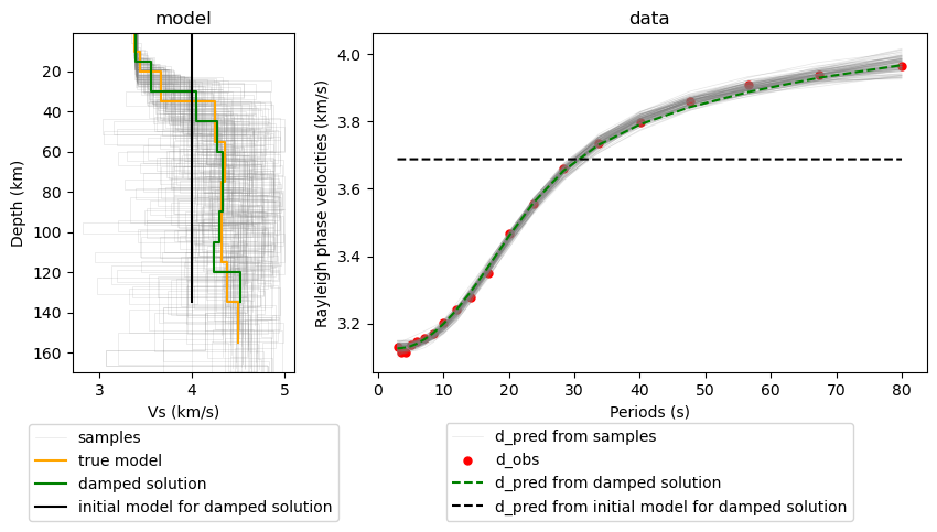
# plot the model and d_pred for starting model
axes = plot_model_and_data(model=init_model, label_model="initial model for damped solution", color_model="black",
                           forward_func=forward_sw, periods=synth_d_periods,
                           label_d_pred="d_pred from initial model for damped solution", color_d_pred="black")

# plot the model and d_pred for true model
plot_model_and_data(model=true_model, label_model="true model", color_model="orange",
                    forward_func=forward_sw, periods=synth_d_periods,
                    label_d_pred="d_pred from true model", color_d_pred="orange", axes=axes)

# plot the model and d_pred for damped solution, and d_obs
plot_model_and_data(model=inv_result_optimiser.model, label_model="damped solution", color_model="green",
                    forward_func=forward_sw, periods=synth_d_periods,
                    label_d_pred="d_pred from damped solution", color_d_pred="green", axes=axes);

# plot randomly selected samples and data predictions from samples
flat_samples = sampler.get_chain(discard=500, thin=500, flat=True)
rand_indices = np.random.randint(len(flat_samples), size=100)
for idx in rand_indices:
    sample = flat_samples[idx]
    label_model = "sample models" if idx == 0 else None
    label_d_pred = "d_pred from samples" if idx == 0 else None
    plot_model_and_data(model=sample, label_model=label_model, color_model="gray",
                        forward_func=forward_sw, periods=synth_d_periods,
                        label_d_pred=label_d_pred, color_d_pred="gray", axes=axes, light_thin=True)

# plot d_obs
plot_data(d_obs, synth_d_periods, ax=axes[1], scatter=True, color="red", s=20, label="d_obs")

axes[0].set_ylim(170)
axes[0].legend(loc="lower center", bbox_to_anchor=(0.5, -0.46))
axes[1].legend(loc="lower center", bbox_to_anchor=(0.5, -0.46));
<matplotlib.legend.Legend object at 0x7efda0e41450>
labels = ["v0", "t0", "v1", "t1", "v2", "t2", "v3", "t3", "v4", "t4", "v5", "t5", "v6", "t6", "v7", "t7", "v8"]

pc = az.plot_trace_dist(
    az_idata,
    visuals={"xlabel_trace": False, "trace": {"color": "C0"}, "dist": {"color": "C0"}},
    figure_kwargs={"figsize": (10, 25), "constrained_layout": True},
)

n_vars = len(az_idata.posterior.data_vars)
var_names = list(az_idata.posterior.data_vars)
for i in range(n_vars):
    ax1 = pc.iget_target(i, 0)
    ax2 = pc.iget_target(i, 1)
    ax1.axvline(true_model[i], linestyle="dotted", color="red")
    ax1.set_title(var_names[i])
    ax1.set_xlabel("parameter value")
    ax1.set_ylabel("density value")
    ax2.set_title(var_names[i])
    ax2.set_xlabel("number of iterations")
    ax2.set_ylabel("parameter value")
    ax2.margins(x=0)
More steps?
Due to time restrictions, we have only run 2_000 steps above, which might be enough for illustration purpose and sanity check, but are not enough for an actual inversion.
On a seperate experiment, we ran 200_000 steps instead and produced the following samples plot.
Fixed-dimensional sampling results with 200_000 steps#
Trans-dimensional sampling#
Prepare utilities for trans-dimensional sampling
def forward_for_bayesbay(state):
    vs = state["voronoi"]["vs"]
    voronoi_sites = state["voronoi"]["discretization"]
    depths = (voronoi_sites[:-1] + voronoi_sites[1:]) / 2
    thicknesses = depths - np.insert(depths[:-1], 0, 0)
    model = form_layercake_model(thicknesses, vs)
    return forward_sw(model, synth_d_periods)
targets = [bayesbay.likelihood.Target("rayleigh", d_obs, covariance_mat_inv=1/noise_level**2)]
fwd_funcs = [forward_for_bayesbay]
my_log_likelihood = bayesbay.likelihood.LogLikelihood(targets, fwd_funcs)
param_vs = bayesbay.prior.UniformPrior(
    name="vs",
    vmin=[2.7, 3.2, 3.75],
    vmax=[4, 4.75, 5],
    position=[0, 40, 80],
    perturb_std=0.15
)

def param_vs_initialize(param, positions):
    vmin, vmax = param.get_vmin_vmax(positions)
    sorted_vals = np.sort(np.random.uniform(vmin, vmax, positions.size))
    for i in range (len(sorted_vals)):
        val = sorted_vals[i]
        vmin_i = vmin if np.isscalar(vmin) else vmin[i]
        vmax_i = vmax if np.isscalar(vmax) else vmax[i]
        if val < vmin_i or val > vmax_i:
            if val > vmax_i: sorted_vals[i] = vmax_i
            if val < vmin_i: sorted_vals[i] = vmin_i
    return sorted_vals

param_vs.set_custom_initialize(param_vs_initialize)
parameterization = bayesbay.parameterization.Parameterization(
    bayesbay.discretization.Voronoi1D(
        name="voronoi",
        vmin=0,
        vmax=150,
        perturb_std=10,
        n_dimensions=None,
        n_dimensions_min=4,
        n_dimensions_max=15,
        parameters=[param_vs],
    )
)
my_perturbation_funcs=parameterization.perturbation_funcs
n_chains=12
walkers_start = []
for i in range(n_chains):
    walkers_start.append(parameterization.initialize())
Define ``InversionOptions``
inv_options_trans_d_sampling = cofi.InversionOptions()
inv_options_trans_d_sampling.set_tool("bayesbay")
inv_options_trans_d_sampling.set_params(
    walkers_starting_states=walkers_start,
    perturbation_funcs=my_perturbation_funcs,
    log_like_ratio_func=my_log_likelihood,
    n_chains=n_chains,
    n_iterations=3_000,
    burnin_iterations=1_000,
    verbose=False,
    save_every=200,
)
Define ``Inversion`` and run
inversion_trans_d_sampler = cofi.Inversion(sw_problem, inv_options_trans_d_sampling)
inv_result_trans_d_sampler = inversion_trans_d_sampler.run()
inverted_models = inv_result_trans_d_sampler.models
samples = []
for v, vs in zip(inverted_models["voronoi.discretization"], inverted_models["voronoi.vs"]):
    sample = form_voronoi_model(v, vs)
    samples.append(voronoi_to_layercake(sample))
# plot the model and d_pred for starting model
axes = plot_model_and_data(model=init_model, label_model="initial model for damped solution", color_model="black",
                           forward_func=forward_sw, periods=synth_d_periods,
                           label_d_pred="d_pred from initial model for damped solution", color_d_pred="black")

# plot the model and d_pred for true model
plot_model_and_data(model=true_model, label_model="true model", color_model="orange",
                    forward_func=forward_sw, periods=synth_d_periods,
                    label_d_pred="d_pred from true model", color_d_pred="orange", axes=axes)

# plot the model and d_pred for damped solution, and d_obs
plot_model_and_data(model=inv_result_optimiser.model, label_model="damped solution", color_model="green",
                    forward_func=forward_sw, periods=synth_d_periods,
                    label_d_pred="d_pred from damped solution", color_d_pred="green", axes=axes);

# plot randomly selected samples and data predictions from samples
for i, sample in enumerate(samples):
    label_model = "sample models" if i == 0 else None
    label_d_pred = "d_pred from samples" if i == 0 else None
    plot_model_and_data(model=sample, label_model=label_model, color_model="gray",
                        forward_func=forward_sw, periods=synth_d_periods,
                        label_d_pred=label_d_pred, color_d_pred="gray", axes=axes, light_thin=True)

# plot d_obs
plot_data(d_obs, synth_d_periods, ax=axes[1], scatter=True, color="red", s=20, label="d_obs")

axes[0].set_ylim(170)
axes[0].legend(loc="lower center", bbox_to_anchor=(0.5, -0.46))
axes[1].legend(loc="lower center", bbox_to_anchor=(0.5, -0.46));
<matplotlib.legend.Legend object at 0x7efda18747d0>
Field data example#
Read data#
Rayleigh observations
file_surf_data = "../../data/sw_rf_joint/data/SURF/nnall.dsp"

with open(file_surf_data, "r") as file:
    lines = file.readlines()
    surf_data = []
    for line in lines:
        row = line.strip().split()
        if "C" in row:
            surf_data.append([float(e) for e in row[5:8]])

field_d = np.array(surf_data)
field_d_periods = field_d[:,0]
field_d_obs = field_d[:,1]
ax = plot_data(field_d_obs, field_d_periods, color="brown", s=5, scatter=True,
             label="d_obs")
ax.legend();
<matplotlib.legend.Legend object at 0x7efdae3d39d0>
Reference good model
file_end_mod = "../../data/sw_rf_joint/data/SURF/end.mod"

with open(file_end_mod, "r") as file:
    lines = file.readlines()
    ref_good_model = []
    for line in lines[12:]:
        row = line.strip().split()
        ref_good_model.append([float(row[0]), float(row[2])])

ref_good_model = np.array(ref_good_model)
ref_good_model = form_layercake_model(ref_good_model[:-1,0], ref_good_model[:,1])
_, ax = plt.subplots(figsize=(4,6))
plot_model(ref_good_model, ax=ax, alpha=1);
<Axes: title={'center': 'model'}, xlabel='Vs (km/s)', ylabel='Depth (km)'>
Modified forward utility#
def forward_sw_interp(model, periods=field_d_periods):
    pysurf_periods = np.logspace(
        np.log(np.min(periods)),
        np.log(np.max(periods+1)),
        60,
        base=np.e,
    )
    pysurf_dpred = forward_sw(model, pysurf_periods)
    interp_func = scipy.interpolate.interp1d(pysurf_periods,
                                             pysurf_dpred,
                                             fill_value="extrapolate")
    dpred = interp_func(periods)
    return dpred
Optimisation#
n_dims = 29

init_thicknesses = np.ones((n_dims//2,)) * 10
init_vs = np.ones((n_dims//2+1,)) * 4.0
init_model = form_layercake_model(init_thicknesses, init_vs)
my_reg = cofi.utils.QuadraticReg(
    weighting_matrix="damping",
    model_shape=(n_dims,),
    reference_model=init_model
)
Optimisation with no damping#
lamda = 0

kwargs = {
    "fwd": forward_sw_interp,
    "periods": field_d_periods,
    "d_obs": field_d_obs,
    "lamda": lamda,
}
sw_field_problem_no_reg = cofi.BaseProblem()
sw_field_problem_no_reg.set_objective(my_objective, kwargs=kwargs)
sw_field_problem_no_reg.set_gradient(my_objective_gradient, kwargs=kwargs)
sw_field_problem_no_reg.set_hessian(my_objective_hessian, kwargs=kwargs)
sw_field_problem_no_reg.set_initial_model(init_model)
Define ``Inversion`` and run
inv_sw_field_problem_no_reg = cofi.Inversion(sw_field_problem_no_reg, inv_options_optimiser)
inv_result_sw_field_no_reg = inv_sw_field_problem_no_reg.run()
Plot results
field_d_periods_logspace = np.logspace(
    np.log(np.min(field_d_periods)),
    np.log(np.max(field_d_periods+1)),
    60,
    base=np.e,
)
# plot the model and d_pred for starting model
axes = plot_model_and_data(model=init_model, label_model="starting model", color_model="black",
                           forward_func=forward_sw_interp, periods=field_d_periods_logspace,
                           label_d_pred="d_pred from starting model", color_d_pred="black")

# plot the model and d_pred for true model
plot_model_and_data(model=ref_good_model, label_model="reference good model", color_model="red",
                    forward_func=forward_sw_interp, periods=field_d_periods_logspace,
                    label_d_pred="d_pred from reference good model", color_d_pred="red", axes=axes)

# plot the model and d_pred for inverted model, and d_obs
plot_model_and_data(model=inv_result_sw_field_no_reg.model,
                    label_model="inverted model from field data", color_model="purple",
                    forward_func=forward_sw_interp, periods=field_d_periods_logspace,
                    label_d_pred="d_pred from inverted model", color_d_pred="purple", axes=axes)

# plot d_obs
plot_data(field_d_obs, field_d_periods, ax=axes[1], scatter=True, color="orange", s=8, label="d_obs")

axes[0].set_ylim(100, 0)
axes[0].legend(loc="lower center", bbox_to_anchor=(0.5, -0.4))
axes[1].legend(loc="lower center", bbox_to_anchor=(0.5, -0.46));
<matplotlib.legend.Legend object at 0x7efdae3d1d10>
Optimal damping#
Again, we would like to find a good regularisation factor.
lambdas = np.logspace(-6, 6, 15)

my_lcurve_problems = []
for lamb in lambdas:
    my_problem = cofi.BaseProblem()
    kwargs = {
        "fwd": forward_sw_interp,
        "periods": field_d_periods,
        "d_obs": field_d_obs,
        "lamda": lamb,
    }
    my_problem.set_objective(my_objective, kwargs=kwargs)
    my_problem.set_gradient(my_objective_gradient, kwargs=kwargs)
    my_problem.set_hessian(my_objective_hessian, kwargs=kwargs)
    my_problem.set_initial_model(init_model)
    my_lcurve_problems.append(my_problem)

def my_callback(inv_result, i):
    m = inv_result.model
    res_norm = np.linalg.norm(forward_sw_interp(m, field_d_periods) - field_d_obs)
    reg_norm = np.sqrt(my_reg(m))
    print(f"Finished inversion with lambda={lambdas[i]}: {res_norm}, {reg_norm}")
    return res_norm, reg_norm

my_inversion_pool = cofi.utils.InversionPool(
    list_of_inv_problems=my_lcurve_problems,
    list_of_inv_options=inv_options_optimiser,
    callback=my_callback,
    parallel=False
)
all_res, all_cb_returns = my_inversion_pool.run()

l_curve_points = list(zip(*all_cb_returns))
Finished inversion with lambda=1e-06: 1.985114475403252, 4.004926608005875
Finished inversion with lambda=7.196856730011514e-06: 1.9856165431508779, 3.9687874809723316
Finished inversion with lambda=5.1794746792312125e-05: 1.9847536060678685, 4.052138855002516
Finished inversion with lambda=0.0003727593720314938: 1.985206668613372, 3.9728860914856043
Finished inversion with lambda=0.0026826957952797246: 1.9844143859178365, 3.9343057695909383
Finished inversion with lambda=0.019306977288832496: 2.00504875898313, 2.3444829711502253
Finished inversion with lambda=0.1389495494373136: 2.039307560040077, 1.6477196400618837
Finished inversion with lambda=1.0: 2.1129352066202585, 1.3870389626598723
Finished inversion with lambda=7.196856730011514: 2.7878709628525176, 0.9907596195990269
Finished inversion with lambda=51.79474679231202: 4.890121206314141, 0.34475341704573875
Finished inversion with lambda=372.7593720314938: 5.957317958789923, 0.06130040191481636
Finished inversion with lambda=2682.6957952797275: 6.160090401090758, 0.008874082501172824
Finished inversion with lambda=19306.977288832455: 6.189746332507266, 0.0012405710283712814
Finished inversion with lambda=138949.5494373136: 6.193898396141414, 0.00017252347237342765
Finished inversion with lambda=1000000.0: 6.194456571037781, 2.3974367261401122e-05
# print all the lambdas
lambdas
array([1.00000000e-06, 7.19685673e-06, 5.17947468e-05, 3.72759372e-04,
       2.68269580e-03, 1.93069773e-02, 1.38949549e-01, 1.00000000e+00,
       7.19685673e+00, 5.17947468e+01, 3.72759372e+02, 2.68269580e+03,
       1.93069773e+04, 1.38949549e+05, 1.00000000e+06])
# plot the L-curve
res_norm, reg_norm = l_curve_points
plt.plot(reg_norm, res_norm, '.-')
plt.xlabel(r'Norm of regularization term $||Wm||_2$')
plt.ylabel(r'Norm of residual $||g(m)-d||_2$')
for i in range(0, len(lambdas), 2):
    plt.annotate(f'{lambdas[i]:.1e}', (reg_norm[i], res_norm[i]), fontsize=8)
Optimisation with damping#
lamda = 0.14

kwargs = {
    "fwd": forward_sw_interp,
    "periods": field_d_periods,
    "d_obs": field_d_obs,
    "lamda": lamda,
}
sw_field_problem = cofi.BaseProblem()
sw_field_problem.set_objective(my_objective, kwargs=kwargs)
sw_field_problem.set_gradient(my_objective_gradient, kwargs=kwargs)
sw_field_problem.set_hessian(my_objective_hessian, kwargs=kwargs)
sw_field_problem.set_initial_model(init_model)
Define ``Inversion`` and run
inv_sw_field_problem = cofi.Inversion(sw_field_problem, inv_options_optimiser)
inv_result_sw_field = inv_sw_field_problem.run()
Plot results
# plot the model and d_pred for starting model
axes = plot_model_and_data(model=init_model, label_model="starting model", color_model="black",
                           forward_func=forward_sw_interp, periods=field_d_periods_logspace,
                           label_d_pred="d_pred from starting model", color_d_pred="black")

# plot the model and d_pred for true model
plot_model_and_data(model=ref_good_model, label_model="reference good model", color_model="red",
                    forward_func=forward_sw_interp, periods=field_d_periods_logspace,
                    label_d_pred="d_pred from reference good model", color_d_pred="red", axes=axes)

# plot the model and d_pred for inverted model, and d_obs
plot_model_and_data(model=inv_result_sw_field.model,
                    label_model="inverted model from field data", color_model="purple",
                    forward_func=forward_sw_interp, periods=field_d_periods_logspace,
                    label_d_pred="d_pred from inverted model", color_d_pred="purple", axes=axes)

# plot d_obs
plot_data(field_d_obs, field_d_periods, ax=axes[1], scatter=True, color="orange", s=8, label="d_obs")

axes[0].set_ylim(100, 0)
axes[0].legend(loc="lower center", bbox_to_anchor=(0.5, -0.4))
axes[1].legend(loc="lower center", bbox_to_anchor=(0.5, -0.46));
<matplotlib.legend.Legend object at 0x7efda1712d50>
Fixed-dimensional sampling#
We are going to use the same sets of log prior, and we will rewrite the log likelihood function to apply on the field data.
thick_min = 3
thick_max = 10
vs_min = 2
vs_max = 5.5

def my_log_prior(model):
    thicknesses, vs = split_layercake_model(model)
    thicknesses_out_of_bounds = (thicknesses < thick_min) | (thicknesses > thick_max)
    vs_out_of_bounds = (vs < vs_min) | (vs > vs_max)
    if np.any(thicknesses_out_of_bounds) or np.any(vs_out_of_bounds):
        return float("-inf")
    log_prior = - np.log(thick_max - thick_min) * len(thicknesses) \
                - np.log(vs_max - vs_min) * len(vs)
    return log_prior
# estimate the data noise
d_pred_from_optimiser = forward_sw_interp(inv_result_sw_field.model, field_d_periods)
noise_level = np.std(field_d_obs - d_pred_from_optimiser)
Cdinv = np.eye(len(field_d_obs))/(noise_level**2)

print(f"Estimated noise level: {noise_level}")
Estimated noise level: 0.10587819642203654
def my_log_likelihood(model):
    try:
        d_pred = forward_sw_interp(model, field_d_periods)
    except:
        return float("-inf")
    residual = field_d_obs - d_pred
    return -0.5 * residual @ (Cdinv @ residual).T
n_walkers = 60

my_walkers_start = np.ones((n_walkers, n_dims)) * inv_result_sw_field.model
for i in range(n_walkers):
    my_walkers_start[i,:] += np.random.normal(0, 0.3, n_dims)
sw_field_problem.set_log_prior(my_log_prior)
sw_field_problem.set_log_likelihood(my_log_likelihood)
Define ``InversionOptions``
inv_options_fixed_d_sampling = cofi.InversionOptions()
inv_options_fixed_d_sampling.set_tool("emcee")
inv_options_fixed_d_sampling.set_params(
    nwalkers=n_walkers,
    nsteps=20_000,
    initial_state=my_walkers_start,
    skip_initial_state_check=True,
    progress=True
)
Sample the posterior#
inversion_fixed_d_sampler_field = cofi.Inversion(sw_field_problem,
                                                 inv_options_fixed_d_sampling)
inv_result_fixed_d_sampler_field = inversion_fixed_d_sampler_field.run()
  0%|          | 0/20000 [00:00<?, ?it/s]
  0%|          | 92/20000 [00:00<00:21, 913.57it/s]
  1%|          | 186/20000 [00:00<00:21, 923.62it/s]
  1%|▏         | 279/20000 [00:00<00:21, 922.33it/s]
  2%|▏         | 373/20000 [00:00<00:21, 929.24it/s]
  2%|▏         | 466/20000 [00:00<00:21, 926.35it/s]
  3%|▎         | 560/20000 [00:00<00:20, 928.44it/s]
  3%|▎         | 653/20000 [00:00<00:20, 928.24it/s]
  4%|▎         | 746/20000 [00:00<00:21, 916.58it/s]
  4%|▍         | 838/20000 [00:00<00:21, 895.74it/s]
  5%|▍         | 928/20000 [00:01<00:21, 894.86it/s]
  5%|▌         | 1022/20000 [00:01<00:20, 906.49it/s]
  6%|▌         | 1115/20000 [00:01<00:20, 913.01it/s]
  6%|▌         | 1208/20000 [00:01<00:20, 918.09it/s]
  7%|▋         | 1303/20000 [00:01<00:20, 924.84it/s]
  7%|▋         | 1396/20000 [00:01<00:20, 925.74it/s]
  7%|▋         | 1490/20000 [00:01<00:19, 927.25it/s]
  8%|▊         | 1585/20000 [00:01<00:19, 932.64it/s]
  8%|▊         | 1679/20000 [00:01<00:19, 931.51it/s]
  9%|▉         | 1773/20000 [00:01<00:19, 931.86it/s]
  9%|▉         | 1867/20000 [00:02<00:19, 931.02it/s]
 10%|▉         | 1961/20000 [00:02<00:19, 933.57it/s]
 10%|█         | 2055/20000 [00:02<00:19, 934.94it/s]
 11%|█         | 2149/20000 [00:02<00:19, 935.20it/s]
 11%|█         | 2243/20000 [00:02<00:18, 936.22it/s]
 12%|█▏        | 2337/20000 [00:02<00:18, 932.79it/s]
 12%|█▏        | 2431/20000 [00:02<00:18, 929.79it/s]
 13%|█▎        | 2525/20000 [00:02<00:18, 931.93it/s]
 13%|█▎        | 2620/20000 [00:02<00:18, 935.63it/s]
 14%|█▎        | 2715/20000 [00:02<00:18, 939.61it/s]
 14%|█▍        | 2809/20000 [00:03<00:18, 939.09it/s]
 15%|█▍        | 2904/20000 [00:03<00:18, 940.10it/s]
 15%|█▍        | 2999/20000 [00:03<00:18, 942.30it/s]
 15%|█▌        | 3094/20000 [00:03<00:18, 934.72it/s]
 16%|█▌        | 3188/20000 [00:03<00:17, 935.65it/s]
 16%|█▋        | 3283/20000 [00:03<00:17, 937.37it/s]
 17%|█▋        | 3378/20000 [00:03<00:17, 939.06it/s]
 17%|█▋        | 3474/20000 [00:03<00:17, 943.38it/s]
 18%|█▊        | 3569/20000 [00:03<00:17, 943.07it/s]
 18%|█▊        | 3664/20000 [00:03<00:17, 944.72it/s]
 19%|█▉        | 3759/20000 [00:04<00:17, 940.39it/s]
 19%|█▉        | 3855/20000 [00:04<00:17, 944.51it/s]
 20%|█▉        | 3950/20000 [00:04<00:17, 942.09it/s]
 20%|██        | 4045/20000 [00:04<00:16, 942.73it/s]
 21%|██        | 4140/20000 [00:04<00:16, 940.81it/s]
 21%|██        | 4235/20000 [00:04<00:16, 938.61it/s]
 22%|██▏       | 4329/20000 [00:04<00:17, 916.99it/s]
 22%|██▏       | 4421/20000 [00:04<00:17, 906.48it/s]
 23%|██▎       | 4514/20000 [00:04<00:16, 911.25it/s]
 23%|██▎       | 4606/20000 [00:04<00:16, 911.18it/s]
 23%|██▎       | 4699/20000 [00:05<00:16, 914.98it/s]
 24%|██▍       | 4794/20000 [00:05<00:16, 924.67it/s]
 24%|██▍       | 4890/20000 [00:05<00:16, 932.47it/s]
 25%|██▍       | 4984/20000 [00:05<00:16, 934.54it/s]
 25%|██▌       | 5078/20000 [00:05<00:15, 934.31it/s]
 26%|██▌       | 5173/20000 [00:05<00:15, 938.47it/s]
 26%|██▋       | 5268/20000 [00:05<00:15, 941.09it/s]
 27%|██▋       | 5363/20000 [00:05<00:15, 936.36it/s]
 27%|██▋       | 5458/20000 [00:05<00:15, 937.96it/s]
 28%|██▊       | 5552/20000 [00:05<00:15, 916.33it/s]
 28%|██▊       | 5644/20000 [00:06<00:15, 900.85it/s]
 29%|██▊       | 5737/20000 [00:06<00:15, 909.02it/s]
 29%|██▉       | 5831/20000 [00:06<00:15, 916.87it/s]
 30%|██▉       | 5924/20000 [00:06<00:15, 919.51it/s]
 30%|███       | 6017/20000 [00:06<00:15, 922.53it/s]
 31%|███       | 6113/20000 [00:06<00:14, 932.57it/s]
 31%|███       | 6208/20000 [00:06<00:14, 935.34it/s]
 32%|███▏      | 6303/20000 [00:06<00:14, 937.37it/s]
 32%|███▏      | 6399/20000 [00:06<00:14, 943.03it/s]
 32%|███▏      | 6494/20000 [00:06<00:14, 942.95it/s]
 33%|███▎      | 6590/20000 [00:07<00:14, 945.85it/s]
 33%|███▎      | 6685/20000 [00:07<00:14, 945.72it/s]
 34%|███▍      | 6781/20000 [00:07<00:13, 949.82it/s]
 34%|███▍      | 6877/20000 [00:07<00:13, 951.14it/s]
 35%|███▍      | 6973/20000 [00:07<00:13, 950.52it/s]
 35%|███▌      | 7069/20000 [00:07<00:13, 952.49it/s]
 36%|███▌      | 7165/20000 [00:07<00:13, 952.25it/s]
 36%|███▋      | 7261/20000 [00:07<00:13, 950.82it/s]
 37%|███▋      | 7357/20000 [00:07<00:13, 949.35it/s]
 37%|███▋      | 7452/20000 [00:07<00:13, 948.46it/s]
 38%|███▊      | 7547/20000 [00:08<00:13, 944.66it/s]
 38%|███▊      | 7642/20000 [00:08<00:13, 940.72it/s]
 39%|███▊      | 7737/20000 [00:08<00:13, 939.01it/s]
 39%|███▉      | 7832/20000 [00:08<00:12, 941.82it/s]
 40%|███▉      | 7928/20000 [00:08<00:12, 946.42it/s]
 40%|████      | 8023/20000 [00:08<00:12, 941.81it/s]
 41%|████      | 8118/20000 [00:08<00:12, 934.88it/s]
 41%|████      | 8214/20000 [00:08<00:12, 939.72it/s]
 42%|████▏     | 8309/20000 [00:08<00:12, 942.68it/s]
 42%|████▏     | 8404/20000 [00:09<00:12, 941.81it/s]
 42%|████▏     | 8499/20000 [00:09<00:12, 940.21it/s]
 43%|████▎     | 8594/20000 [00:09<00:12, 938.80it/s]
 43%|████▎     | 8688/20000 [00:09<00:12, 937.95it/s]
 44%|████▍     | 8784/20000 [00:09<00:11, 942.96it/s]
 44%|████▍     | 8879/20000 [00:09<00:11, 943.29it/s]
 45%|████▍     | 8975/20000 [00:09<00:11, 946.21it/s]
 45%|████▌     | 9070/20000 [00:09<00:11, 929.54it/s]
 46%|████▌     | 9164/20000 [00:09<00:11, 920.60it/s]
 46%|████▋     | 9257/20000 [00:09<00:11, 923.13it/s]
 47%|████▋     | 9353/20000 [00:10<00:11, 932.39it/s]
 47%|████▋     | 9447/20000 [00:10<00:11, 934.29it/s]
 48%|████▊     | 9543/20000 [00:10<00:11, 938.99it/s]
 48%|████▊     | 9639/20000 [00:10<00:10, 943.76it/s]
 49%|████▊     | 9734/20000 [00:10<00:10, 942.11it/s]
 49%|████▉     | 9830/20000 [00:10<00:10, 945.34it/s]
 50%|████▉     | 9925/20000 [00:10<00:10, 941.81it/s]
 50%|█████     | 10020/20000 [00:10<00:10, 941.02it/s]
 51%|█████     | 10115/20000 [00:10<00:10, 935.68it/s]
 51%|█████     | 10211/20000 [00:10<00:10, 940.23it/s]
 52%|█████▏    | 10306/20000 [00:11<00:10, 930.41it/s]
 52%|█████▏    | 10400/20000 [00:11<00:10, 921.90it/s]
 52%|█████▏    | 10494/20000 [00:11<00:10, 924.87it/s]
 53%|█████▎    | 10589/20000 [00:11<00:10, 931.11it/s]
 53%|█████▎    | 10683/20000 [00:11<00:10, 927.35it/s]
 54%|█████▍    | 10777/20000 [00:11<00:09, 930.54it/s]
 54%|█████▍    | 10871/20000 [00:11<00:09, 933.25it/s]
 55%|█████▍    | 10966/20000 [00:11<00:09, 937.69it/s]
 55%|█████▌    | 11063/20000 [00:11<00:09, 947.07it/s]
 56%|█████▌    | 11160/20000 [00:11<00:09, 951.37it/s]
 56%|█████▋    | 11256/20000 [00:12<00:09, 952.57it/s]
 57%|█████▋    | 11352/20000 [00:12<00:09, 953.47it/s]
 57%|█████▋    | 11448/20000 [00:12<00:08, 953.63it/s]
 58%|█████▊    | 11544/20000 [00:12<00:08, 949.98it/s]
 58%|█████▊    | 11640/20000 [00:12<00:08, 944.54it/s]
 59%|█████▊    | 11737/20000 [00:12<00:08, 950.32it/s]
 59%|█████▉    | 11833/20000 [00:12<00:08, 951.57it/s]
 60%|█████▉    | 11930/20000 [00:12<00:08, 955.39it/s]
 60%|██████    | 12026/20000 [00:12<00:08, 955.80it/s]
 61%|██████    | 12122/20000 [00:12<00:08, 954.65it/s]
 61%|██████    | 12219/20000 [00:13<00:08, 957.73it/s]
 62%|██████▏   | 12315/20000 [00:13<00:08, 956.59it/s]
 62%|██████▏   | 12411/20000 [00:13<00:07, 957.49it/s]
 63%|██████▎   | 12508/20000 [00:13<00:07, 959.30it/s]
 63%|██████▎   | 12604/20000 [00:13<00:07, 955.92it/s]
 64%|██████▎   | 12700/20000 [00:13<00:07, 954.51it/s]
 64%|██████▍   | 12796/20000 [00:13<00:07, 954.72it/s]
 64%|██████▍   | 12892/20000 [00:13<00:07, 954.67it/s]
 65%|██████▍   | 12989/20000 [00:13<00:07, 958.04it/s]
 65%|██████▌   | 13086/20000 [00:13<00:07, 959.36it/s]
 66%|██████▌   | 13182/20000 [00:14<00:07, 955.61it/s]
 66%|██████▋   | 13278/20000 [00:14<00:07, 956.59it/s]
 67%|██████▋   | 13374/20000 [00:14<00:06, 952.92it/s]
 67%|██████▋   | 13470/20000 [00:14<00:06, 949.90it/s]
 68%|██████▊   | 13565/20000 [00:14<00:06, 946.82it/s]
 68%|██████▊   | 13662/20000 [00:14<00:06, 950.84it/s]
 69%|██████▉   | 13759/20000 [00:14<00:06, 954.28it/s]
 69%|██████▉   | 13855/20000 [00:14<00:06, 948.61it/s]
 70%|██████▉   | 13950/20000 [00:14<00:06, 942.23it/s]
 70%|███████   | 14045/20000 [00:14<00:06, 926.26it/s]
 71%|███████   | 14139/20000 [00:15<00:06, 928.86it/s]
 71%|███████   | 14235/20000 [00:15<00:06, 937.91it/s]
 72%|███████▏  | 14332/20000 [00:15<00:05, 946.07it/s]
 72%|███████▏  | 14429/20000 [00:15<00:05, 950.54it/s]
 73%|███████▎  | 14526/20000 [00:15<00:05, 954.35it/s]
 73%|███████▎  | 14623/20000 [00:15<00:05, 956.06it/s]
 74%|███████▎  | 14720/20000 [00:15<00:05, 958.11it/s]
 74%|███████▍  | 14817/20000 [00:15<00:05, 959.51it/s]
 75%|███████▍  | 14913/20000 [00:15<00:05, 956.27it/s]
 75%|███████▌  | 15009/20000 [00:15<00:05, 956.47it/s]
 76%|███████▌  | 15106/20000 [00:16<00:05, 957.98it/s]
 76%|███████▌  | 15203/20000 [00:16<00:04, 961.05it/s]
 76%|███████▋  | 15300/20000 [00:16<00:04, 962.05it/s]
 77%|███████▋  | 15397/20000 [00:16<00:04, 958.18it/s]
 77%|███████▋  | 15494/20000 [00:16<00:04, 960.12it/s]
 78%|███████▊  | 15591/20000 [00:16<00:04, 960.15it/s]
 78%|███████▊  | 15688/20000 [00:16<00:04, 958.89it/s]
 79%|███████▉  | 15784/20000 [00:16<00:04, 956.45it/s]
 79%|███████▉  | 15881/20000 [00:16<00:04, 957.86it/s]
 80%|███████▉  | 15977/20000 [00:16<00:04, 956.34it/s]
 80%|████████  | 16074/20000 [00:17<00:04, 958.11it/s]
 81%|████████  | 16170/20000 [00:17<00:03, 957.59it/s]
 81%|████████▏ | 16266/20000 [00:17<00:03, 955.94it/s]
 82%|████████▏ | 16362/20000 [00:17<00:03, 955.46it/s]
 82%|████████▏ | 16459/20000 [00:17<00:03, 957.15it/s]
 83%|████████▎ | 16556/20000 [00:17<00:03, 960.65it/s]
 83%|████████▎ | 16653/20000 [00:17<00:03, 959.52it/s]
 84%|████████▍ | 16750/20000 [00:17<00:03, 960.07it/s]
 84%|████████▍ | 16847/20000 [00:17<00:03, 958.48it/s]
 85%|████████▍ | 16944/20000 [00:18<00:03, 961.52it/s]
 85%|████████▌ | 17041/20000 [00:18<00:03, 957.32it/s]
 86%|████████▌ | 17138/20000 [00:18<00:02, 958.27it/s]
 86%|████████▌ | 17235/20000 [00:18<00:02, 959.20it/s]
 87%|████████▋ | 17332/20000 [00:18<00:02, 960.90it/s]
 87%|████████▋ | 17429/20000 [00:18<00:02, 962.76it/s]
 88%|████████▊ | 17526/20000 [00:18<00:02, 961.37it/s]
 88%|████████▊ | 17623/20000 [00:18<00:02, 960.59it/s]
 89%|████████▊ | 17720/20000 [00:18<00:02, 961.21it/s]
 89%|████████▉ | 17817/20000 [00:18<00:02, 950.85it/s]
 90%|████████▉ | 17913/20000 [00:19<00:02, 941.34it/s]
 90%|█████████ | 18008/20000 [00:19<00:02, 943.50it/s]
 91%|█████████ | 18103/20000 [00:19<00:02, 941.43it/s]
 91%|█████████ | 18198/20000 [00:19<00:01, 938.70it/s]
 91%|█████████▏| 18294/20000 [00:19<00:01, 942.77it/s]
 92%|█████████▏| 18389/20000 [00:19<00:01, 938.25it/s]
 92%|█████████▏| 18484/20000 [00:19<00:01, 940.92it/s]
 93%|█████████▎| 18580/20000 [00:19<00:01, 943.32it/s]
 93%|█████████▎| 18676/20000 [00:19<00:01, 947.65it/s]
 94%|█████████▍| 18771/20000 [00:19<00:01, 937.02it/s]
 94%|█████████▍| 18865/20000 [00:20<00:01, 912.52it/s]
 95%|█████████▍| 18960/20000 [00:20<00:01, 922.07it/s]
 95%|█████████▌| 19055/20000 [00:20<00:01, 929.71it/s]
 96%|█████████▌| 19149/20000 [00:20<00:00, 931.46it/s]
 96%|█████████▌| 19244/20000 [00:20<00:00, 936.03it/s]
 97%|█████████▋| 19340/20000 [00:20<00:00, 941.71it/s]
 97%|█████████▋| 19437/20000 [00:20<00:00, 949.06it/s]
 98%|█████████▊| 19533/20000 [00:20<00:00, 950.92it/s]
 98%|█████████▊| 19629/20000 [00:20<00:00, 949.29it/s]
 99%|█████████▊| 19724/20000 [00:20<00:00, 944.13it/s]
 99%|█████████▉| 19820/20000 [00:21<00:00, 947.58it/s]
100%|█████████▉| 19915/20000 [00:21<00:00, 948.14it/s]
100%|██████████| 20000/20000 [00:21<00:00, 941.52it/s]
sampler = inv_result_fixed_d_sampler.sampler
az_idata = az.from_emcee(sampler, var_names=labels)
az_idata.get("posterior")
# plot the model and d_pred for starting model
axes = plot_model_and_data(model=init_model, label_model="starting model", color_model="black",
                           forward_func=forward_sw_interp, periods=field_d_periods_logspace,
                           label_d_pred="d_pred from starting model", color_d_pred="black")

# plot the model and d_pred for true model
plot_model_and_data(model=ref_good_model, label_model="reference good model", color_model="red",
                    forward_func=forward_sw_interp, periods=field_d_periods_logspace,
                    label_d_pred="d_pred from reference good model", color_d_pred="red", axes=axes)

# plot the model and d_pred for inverted model, and d_obs
plot_model_and_data(model=inv_result_sw_field.model,
                    label_model="inverted model from field data", color_model="green",
                    forward_func=forward_sw_interp, periods=field_d_periods_logspace,
                    label_d_pred="d_pred from inverted model", color_d_pred="green", axes=axes)

# plot randomly selected samples and data predictions from samples
flat_samples = sampler.get_chain(discard=1000, thin=300, flat=True)
rand_indices = np.random.randint(len(flat_samples), size=100)
for idx in rand_indices:
    sample = flat_samples[idx]
    label_model = "sample models" if idx == 0 else None
    label_d_pred = "d_pred from samples" if idx == 0 else None
    plot_model_and_data(model=sample, label_model=label_model, color_model="gray",
                        forward_func=forward_sw_interp, periods=field_d_periods_logspace,
                        label_d_pred=label_d_pred, color_d_pred="gray", axes=axes, light_thin=True)

# plot d_obs
plot_data(field_d_obs, field_d_periods, ax=axes[1], scatter=True, color="orange", s=8, label="d_obs")

axes[0].set_ylim(100, 0)
axes[0].legend(loc="lower center", bbox_to_anchor=(0.5, -0.4))
axes[1].legend(loc="lower center", bbox_to_anchor=(0.5, -0.46));
<matplotlib.legend.Legend object at 0x7efda67e6710>
More steps
Similar to our earlier fixed-dimensional sampling run on the synthetic data, we are not sampling enough due to time limit.
On a seperate experiment, we ran 200_000 steps and produced the following samples plot.
Trans-dimensional sampling#
def forward_interp_for_bayesbay(state):
    vs = state["voronoi"]["vs"]
    voronoi_sites = state["voronoi"]["discretization"]
    depths = (voronoi_sites[:-1] + voronoi_sites[1:]) / 2
    thicknesses = depths - np.insert(depths[:-1], 0, 0)
    model = form_layercake_model(thicknesses, vs)
    return forward_sw_interp(model, field_d_periods)
targets = [bayesbay.likelihood.Target("rayleigh", field_d_obs, covariance_mat_inv=1/noise_level**2)]
fwd_funcs = [forward_interp_for_bayesbay]
my_log_likelihood = bayesbay.likelihood.LogLikelihood(targets, fwd_funcs)
param_vs = bayesbay.prior.UniformPrior(
    name="vs",
    vmin=[2.7, 3.2, 3.75],
    vmax=[4, 4.75, 5],
    position=[0, 40, 80],
    perturb_std=0.15
)

def param_vs_initialize(param, positions):
    vmin, vmax = param.get_vmin_vmax(positions)
    sorted_vals = np.sort(np.random.uniform(vmin, vmax, positions.size))
    for i in range (len(sorted_vals)):
        val = sorted_vals[i]
        vmin_i = vmin if np.isscalar(vmin) else vmin[i]
        vmax_i = vmax if np.isscalar(vmax) else vmax[i]
        if val < vmin_i or val > vmax_i:
            if val > vmax_i: sorted_vals[i] = vmax_i
            if val < vmin_i: sorted_vals[i] = vmin_i
    return sorted_vals

param_vs.set_custom_initialize(param_vs_initialize)
parameterization = bayesbay.parameterization.Parameterization(
    bayesbay.discretization.Voronoi1D(
        name="voronoi",
        vmin=0,
        vmax=150,
        perturb_std=10,
        n_dimensions=None,
        n_dimensions_min=4,
        n_dimensions_max=20,
        parameters=[param_vs],
    )
)
my_perturbation_funcs = parameterization.perturbation_funcs
n_chains=12
walkers_start = []
for i in range(n_chains):
    walkers_start.append(parameterization.initialize())
Define ``InversionOptions``
inv_options_field_trans_d_sampling = cofi.InversionOptions()
inv_options_field_trans_d_sampling.set_tool("bayesbay")
inv_options_field_trans_d_sampling.set_params(
    walkers_starting_states=walkers_start,
    perturbation_funcs=my_perturbation_funcs,
    log_like_ratio_func=my_log_likelihood,
    n_chains=n_chains,
    n_iterations=3_000,
    burnin_iterations=1_000,
    verbose=False,
    save_every=200,
)
Define ``Inversion`` and run
inversion_field_trans_d_sampler = cofi.Inversion(sw_field_problem,
                                                 inv_options_field_trans_d_sampling)
inv_result_field_trans_d_sampler = inversion_field_trans_d_sampler.run()
inverted_models = inv_result_field_trans_d_sampler.models
samples = []
for v, vs in zip(inverted_models["voronoi.discretization"], inverted_models["voronoi.vs"]):
    sample = form_voronoi_model(v, vs)
    samples.append(voronoi_to_layercake(sample))
# plot the model and d_pred for starting model
axes = plot_model_and_data(model=init_model, label_model="starting model", color_model="black",
                           forward_func=forward_sw_interp, periods=field_d_periods_logspace,
                           label_d_pred="d_pred from starting model", color_d_pred="black")

# plot the model and d_pred for true model
plot_model_and_data(model=ref_good_model, label_model="reference good model", color_model="red",
                    forward_func=forward_sw_interp, periods=field_d_periods_logspace,
                    label_d_pred="d_pred from reference good model", color_d_pred="red", axes=axes)

# plot the model and d_pred for inverted model, and d_obs
plot_model_and_data(model=inv_result_sw_field.model,
                    label_model="inverted model from field data", color_model="green",
                    forward_func=forward_sw_interp, periods=field_d_periods_logspace,
                    label_d_pred="d_pred from inverted model", color_d_pred="green", axes=axes)

# plot randomly selected samples and data predictions from samples
flat_samples = sampler.get_chain(discard=1000, thin=300, flat=True)
rand_indices = np.random.randint(len(flat_samples), size=100)
for i, sample in enumerate(samples):
    label_model = "sample models" if i == 0 else None
    label_d_pred = "d_pred from samples" if i == 0 else None
    plot_model_and_data(model=sample, label_model=label_model, color_model="gray",
                        forward_func=forward_sw_interp, periods=field_d_periods_logspace,
                        label_d_pred=label_d_pred, color_d_pred="gray", axes=axes, light_thin=True)

# plot d_obs
plot_data(field_d_obs, field_d_periods, ax=axes[1], scatter=True, color="orange", s=8, label="d_obs")

axes[0].set_ylim(100, 0)
axes[0].legend(loc="lower center", bbox_to_anchor=(0.5, -0.4))
axes[1].legend(loc="lower center", bbox_to_anchor=(0.5, -0.46));
<matplotlib.legend.Legend object at 0x7efd95cde210>
Watermark#
watermark_list = ["cofi", "numpy", "matplotlib", "scipy", "emcee", "bayesbay"]
for pkg in watermark_list:
    pkg_var = __import__(pkg)
    print(pkg, getattr(pkg_var, "__version__"))
cofi 0.2.11+71.gb28b5b0
numpy 2.2.6
matplotlib 3.10.9
scipy 1.17.1
emcee 3.1.6
bayesbay 0.3.10
sphinx_gallery_thumbnail_number = -1
Total running time of the script: (2 minutes 7.011 seconds)