Note
Go to the end to download the full example code
Linear regression with Eustatic Sea-level data#
If you are running this notebook locally, make sure you’ve followed steps here to set up the environment. (This environment.yml file specifies a list of packages required to run the notebooks)
What we do in this notebook#
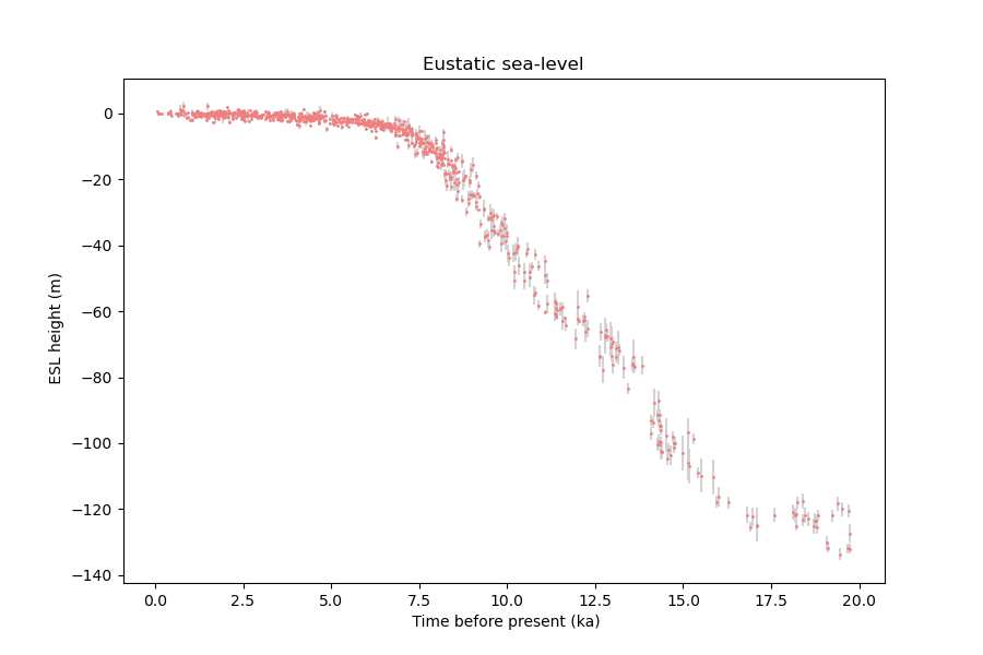
Here we demonstrate use of CoFI on a real dataset linear regression problem, where we fit a polynomial function to Eustatic Sea-level heights.
by solution of a linear system of equations,
by optimization of a data misfit function
by Bayesian sampling of a Likelihood multiplied by a prior.
Data set is from “Sea level and global ice volumes from the Last Glacial Maximum to the Holocene” K. Lambeck, H. Rouby, A. Purcell, Y. Sun, and M. Sambridge, 2014. Proc. Nat. Acad. Sci., 111, no. 43, 15296-15303, doi:10.1073/pnas.1411762111.
# Environment setup (uncomment code below)

# !pip install -U cofi
# !git clone https://github.com/inlab-geo/cofi-examples.git
# %cd cofi-examples/examples/linear_regression
Linear regression#
Lets start with some (x,y) data.
import numpy as np
import matplotlib.pyplot as plt
#
def load_data_xy(filename):

    f = open(filename, 'r')
    header = f.readline()
    lines = f.readlines()

    x = np.array([])
    y = np.array([])
    sx = np.array([])
    sy = np.array([])
    for line in lines:
        columns = line.split()
        x = np.append(x,float(columns[0]))
        y = np.append(y,float(columns[1]))
        sx = np.append(sx,float(columns[2])/2.0)
        sy = np.append(sy,float(columns[3])/2.0)

    d = x,y, sy                                   # Combine into a single data structure

    return d

def load_data_ref(filename):

    f = open(filename, 'r')
    lines = f.readlines()
    dx = np.array([]) # Age data
    dy = np.array([]) # ESL height
    dz = np.array([]) # derivative of ESL w.r.t. age
    for line in lines:
        columns = line.split()
        dx = np.append(dx,float(columns[0]))
        dy = np.append(dy,float(columns[1]))
    datavals = np.column_stack((dx,dy))  # Stack data

    return datavals
And now lets plot the data.
def plot_data(x=data_x,y=data_y,sigma=sy,title=None):
    fig, axes = plt.subplots(figsize=(9,6))
    plt.errorbar(x, y, yerr=sy, fmt='.',color="lightcoral",ecolor='lightgrey',ms=2)
    plt.xlabel(' Time before present (ka)')
    plt.ylabel(' ESL height (m)')
    if(title != None): plt.title(title)
plot_data(title='Eustatic sea-level')
Problem description#
To begin with, we will work with polynomial curves,
Here, \(M\) is the ‘order’ of the polynomial: if \(M=1\) we have a straight line with 2 parameters, if \(M=2\) it will be a quadratic with 3 parameters, and so on. The \(m_j, (j=0,\dots M)\) are the ‘model coefficients’ that we seek to constrain from the data.
For this class of problem the forward operator takes the following form:
This clearly has the required general form, \(\mathbf{d} =G{\mathbf m}\).
where:
\(\textbf{d}\) is the vector of data values, (\(y_0,y_1,\dots,y_N\));
\(\textbf{m}\) is the vector of model parameters, (\(m_0,m_1,m_2\));
\(G\) is the basis matrix (or design matrix) of this linear regression problem (also called the Jacobian matrix for this linear problem).
We have a set of noisy data values, \(y_i (i=0,\dots,N)\), measured at known locations, \(x_i (i=0,\dots,N)\), and wish to find the best fit degree 3 polynomial.
The function that generated our data is assumed to have independent Gaussian random noise, \({\cal N}(0,\Sigma)\), with \((\Sigma)_{ij} = \delta_{ij}/\sigma_i^2\), where the variance of the noise on each datum, \(\sigma_i^2 (i=1,\dots,N)\), differs between observations and is given.
We now build the Jacobian/G matrix for this problem and define a forward function which simply multiplies \(\mathbf m\) by \(G\).
Define a reference model for later.
Now lets plot the data with the reference curve
# Some plotting utilities
def plot_model(x,y, label, color=None,lw=0.5):
    plt.plot(x, y, color=color or "green", label=label,lw=lw)
    #plt.xlabel("X")
    #plt.ylabel("ESL")
    plt.legend()

def plot_models(models, label="Posterior samples", color="seagreen", alpha=0.1,lw=0.5):
    G = jacobian(data_x)
    plt.plot(data_x, G.dot(models[0]), color=color, label=label, alpha=alpha,lw=lw)
    for m in models:
        plt.plot(data_x, G.dot(m), color=color, alpha=alpha,lw=lw)
    plt.legend()
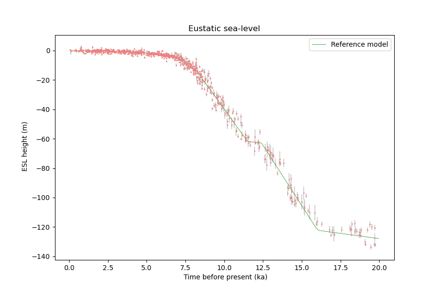
Now we have the data and the forward model we can start to try and estimate the coefficients of the polynomial from the data.
The structure of CoFI#
In the workflow of cofi, there are three main components:
BaseProblem, InversionOptions, and Inversion.
BaseProblemdefines the inverse problem including any user supplied quantities such as data vector, number of model parameters and measure of fit between model predictions and data.python inv_problem = BaseProblem() inv_problem.set_objective(some_function_here) inv_problem.set_jacobian(some_function_here) inv_problem.set_initial_model(a_starting_point) # if needed, e.g. we are solving a nonlinear problem by optimizationInversionOptionsdescribes details about how one wants to run the inversion, including the backend tool and solver-specific parameters. It is based on the concept of amethodandtool.inv_options = InversionOptions() inv_options.suggest_solving_methods() inv_options.set_solving_method("matrix solvers") inv_options.suggest_tools() inv_options.set_tool("scipy.linalg.lstsq") inv_options.summary()
Inversioncan be seen as an inversion engine that takes in the above two as information, and will produce anInversionResultupon running.inv = Inversion(inv_problem, inv_options) result = inv.run()
Internally CoFI decides the nature of the problem from the quantities set by the user and performs internal checks to ensure it has all that it needs to solve a problem.
1. Linear system solver#
from cofi import BaseProblem, InversionOptions, Inversion
Step 1. Define CoFI BaseProblem#
inv_problem = BaseProblem()
inv_problem.set_data(data_y)
inv_problem.set_jacobian(jacobian())
inv_problem.set_data_covariance_inv(Cd_inv())
Step 2. Define CoFI InversionOptions#
inv_options = InversionOptions()
Using the information supplied, we can ask CoFI to suggest some solving methods.
inv_options.suggest_solving_methods()
The following solving methods are supported:
{'sampling', 'optimization', 'matrix solvers'}

Use `suggest_tools()` to see a full list of backend tools for each method
We can ask CoFI to suggest some specific software tools as well.
inv_options.suggest_tools()
Here's a complete list of inversion tools supported by CoFI (grouped by methods):
{
    "optimization": [
        "scipy.optimize.minimize",
        "scipy.optimize.least_squares",
        "torch.optim",
        "cofi.border_collie_optimization"
    ],
    "matrix solvers": [
        "scipy.linalg.lstsq",
        "cofi.simple_newton"
    ],
    "sampling": [
        "emcee",
        "bayesbay",
        "neighpy"
    ]
}
inv_options.set_solving_method("matrix solvers") # lets decide to use a matrix solver.
inv_options.summary()
=============================
Summary for inversion options
=============================
Solving method: matrix solvers
Use `suggest_solving_methods()` to check available solving methods.
-----------------------------
Backend tool: `<class 'cofi.tools._scipy_lstsq.ScipyLstSq'> (by default)` - SciPy's wrapper function over LAPACK's linear least-squares solver, using 'gelsd', 'gelsy' (default), or 'gelss' as backend driver
References: ['https://docs.scipy.org/doc/scipy/reference/generated/scipy.linalg.lstsq.html', 'https://www.netlib.org/lapack/lug/node27.html']
Use `suggest_tools()` to check available backend tools.
-----------------------------
Solver-specific parameters: None set
Use `suggest_solver_params()` to check required/optional solver-specific parameters.
# below is optional, as this has already been the default tool under "linear least square"
inv_options.set_tool("scipy.linalg.lstsq")
Step 3. Define CoFI Inversion and run#
Our choices so far have defined a linear parameter estimation problem
(without any regularization) to be solved within a least squares
framework. In this case the selection of a matrix solvers method
will mean we are calculating the standard least squares solution
and our choice of backend tool scipy.linalg.lstsq, means that we
will employ scipy’s linalg package to perform the numerics.
Lets run CoFI.
inv = Inversion(inv_problem, inv_options)
inv_result = inv.run()
print(f"The inversion result from `scipy.linalg.lstsq`: {inv_result.model}\n")
inv_result.summary()
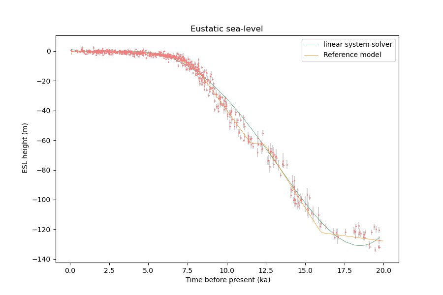
The inversion result from `scipy.linalg.lstsq`: [ 1.44051039 -3.11381469  1.412872   -0.20910136  0.00653572]

============================
Summary for inversion result
============================
SUCCESS
----------------------------
model: [ 1.44051039 -3.11381469  1.412872   -0.20910136  0.00653572]
sum_of_squared_residuals: []
effective_rank: 5
singular_values: [1.72339368e+09 1.35569994e+06 3.54123758e+03 1.10384400e+02
 7.16903392e+00]
model_covariance: [[ 6.70145209e-02 -6.28173834e-02  1.67266578e-02 -1.60867740e-03
   4.77025592e-05]
 [-6.28173834e-02  7.43365995e-02 -2.23488563e-02  2.32179303e-03
  -7.20214235e-05]
 [ 1.67266578e-02 -2.23488563e-02  7.38371078e-03 -8.20763652e-04
   2.65025504e-05]
 [-1.60867740e-03  2.32179303e-03 -8.20763652e-04  9.62437921e-05
  -3.21300646e-06]
 [ 4.77025592e-05 -7.20214235e-05  2.65025504e-05 -3.21300646e-06
   1.10114955e-07]]
Lets plot the solution.
plot_data(title="Eustatic sea-level")
plot_model(data_x,jacobian(data_x).dot(inv_result.model), "linear system solver", color="seagreen")
plot_model(ref_x,ref_y, "Reference model", color="darkorange")
2. Optimizer#
The same overdetermined linear problem, \(\textbf{d} = G\textbf{m}\), with Gaussian data noise can also be solved by minimising the squares of the residual of the linear equations, e.g. \(\textbf{r}^T \textbf{C}_d^{-1}\textbf{r}\) where \(\textbf{r}=\textbf{d}-G\textbf{m}\). The above matrix solver solution gives us the best data fitting model, but a direct optimisation approach could also be used, say when the number of unknowns is large and we do not wish, or are unable to provide the Jacobian function.
So we use a plain optimizer scipy.optimize.minimize to demonstrate
this ability.
######## CoFI BaseProblem - provide additional information
inv_problem.set_initial_model(np.ones(nparams))
#inv_problem.set_initial_model(inv_result.model)
inv_problem.set_forward(forward)
inv_problem.set_data_misfit("squared error")

# inv_problem.set_objective(your_own_misfit_function)    # (optionally) if you'd like to define your own misfit
# inv_problem.set_gradient(your_own_gradient_of_misfit_function)    # (optionally) if you'd like to define your own misfit gradient

######## CoFI InversionOptions - set a different tool
inv_options_2 = InversionOptions()
inv_options_2.set_tool("scipy.optimize.minimize")
inv_options_2.set_params(method="Nelder-Mead")

######## CoFI Inversion - run it
inv_2 = Inversion(inv_problem, inv_options_2)
inv_result_2 = inv_2.run()

######## CoFI InversionResult - check result
print(f"The inversion result from `scipy.optimize.minimize`: {inv_result_2.model}\n")
inv_result_2.summary()
The inversion result from `scipy.optimize.minimize`: [-0.81319113 -0.46081553  0.61740809 -0.12663625  0.00398136]

============================
Summary for inversion result
============================
SUCCESS
----------------------------
fun: 310.0689929995378
nit: 560
nfev: 916
status: 0
message: Optimization terminated successfully.
final_simplex: (array([[-0.81319113, -0.46081553,  0.61740809, -0.12663625,  0.00398136],
       [-0.81328903, -0.46081801,  0.61741429, -0.1266371 ,  0.0039814 ],
       [-0.81317886, -0.46081571,  0.61738786, -0.12663294,  0.00398125],
       [-0.81315239, -0.46081502,  0.61739705, -0.12663469,  0.0039813 ],
       [-0.81320724, -0.46081746,  0.61741117, -0.12663795,  0.00398147],
       [-0.81318091, -0.4608153 ,  0.61740441, -0.12663565,  0.00398136]]), array([310.068993  , 310.06899312, 310.0689937 , 310.06899379,
       310.06899388, 310.06899454]))
model: [-0.81319113 -0.46081553  0.61740809 -0.12663625  0.00398136]
plot_data()
plot_model(data_x,jacobian(data_x).dot(inv_result_2.model), "optimization solution", color="cornflowerblue")
plot_model(ref_x,ref_y, "Reference model", color="darkorange")
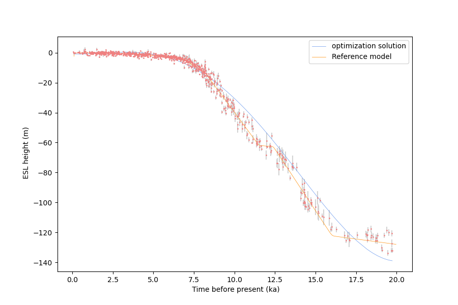
The optimization fails to convergence for this problem (with default settings).
Challenge - Change the polynomial degree#
Try and replace the 3rd order polynomial with a 2nd order polynomial (i.e. \(M=2\)) by adding the required commands below. What does the plot looks like?
Start from code below:
inv_problem = BaseProblem()
inv_problem.set_data(data_y)
inv_problem.set_jacobian(jacobian(n=<CHANGE ME>))
inv_problem.set_data_covariance_inv(Cd_inv())
inv_options.set_solving_method("matrix solvers") # lets decide to use a matrix solver.
inv = Inversion(inv_problem, inv_options)
inv_result = inv.run()

print("Inferred curve with n = <CHANGE ME> ")
plot_data()
plot_model(data_x,jacobian(x,n=<CHANGE ME>).dot(inv_result.model), "optimization solution", color="cornflowerblue")
plot_model(ref_x,ref_y, "Reference model", color="darkorange")
# Copy the template above, Replace <CHANGE ME> with your answer
#@title Solution

inv_problem = BaseProblem()
inv_problem.set_data(data_y)
inv_problem.set_jacobian(jacobian(n=3))
inv_problem.set_data_covariance_inv(Cd_inv())
inv_options.set_solving_method("matrix solvers") # lets decide to use a matrix solver.
inv = Inversion(inv_problem, inv_options)
inv_result = inv.run()

print("Inferred curve with n = 3 ")
plot_data()
plot_model(data_x,jacobian(data_x,n=3).dot(inv_result.model), "optimization solution", color="cornflowerblue")
plot_model(ref_x,ref_y, "Reference model", color="darkorange")
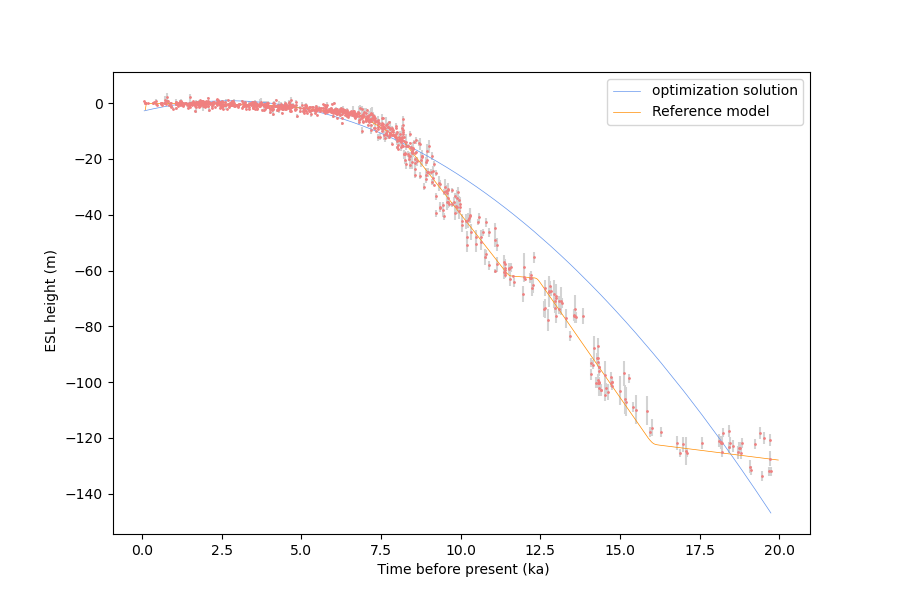
Inferred curve with n = 3
Changing to a second order polynomial does converge but gives a poor fit.
3. Bayesian sampling#
Likelihood#
Since data errors follow a Gaussian in this example, we can define a Likelihood function, \(p({\mathbf d}_{obs}| {\mathbf m})\).
where \({\mathbf d}_{obs}\) represents the observed y values and \({\mathbf d}_{pred}({\mathbf m})\) are those predicted by the polynomial model \(({\mathbf m})\). The Likelihood is defined as the probability of observing the data actually observed, given a model. In practice we usually only need to evaluate the log of the Likelihood, \(\log p({\mathbf d}_{obs} | {\mathbf m})\). To do so, we require the inverse data covariance matrix describing the statistics of the noise in the data, \(C_D^{-1}\) . For this problem the data errors are independent with identical standard deviation in noise for each datum. Hence \(C_D^{-1} = \frac{1}{\sigma^2}I\) where \(\sigma=1\).
Here we artificially increase the observational errors on the data so that the spread of the posterior samples are visible.
Note that the user could specify any appropriate Likelihood function of their choosing here.
Prior#
Bayesian sampling requires a prior probability density function. A common problem with polynomial coefficients as model parameters is that it is not at all obvious what a prior should be. Here we choose a uniform prior with specified bounds
where \(l_i\) and \(u_i\) are lower and upper bounds on the \(i\)th model coefficient.
Here use the uniform distribution with \({\mathbf l}^T = (-10.,-10.,-10.,-10.)\), and \({\mathbf u}^T = (10.,10.,10.,10.)\).
m_lower_bound = np.ones(nparams) * (-10.)             # lower bound for uniform prior
m_upper_bound = np.ones(nparams) * 10                 # upper bound for uniform prior

def log_prior(model):    # uniform distribution
    for i in range(len(m_lower_bound)):
        if model[i] < m_lower_bound[i] or model[i] > m_upper_bound[i]: return -np.inf
    return 0.0 # model lies within bounds -> return log(1)
Note that the user could specify any appropriate Prior PDF of their choosing here.
Bayesian sampling#
In this aproach we sample a probability distribution rather than find a single best fit solution. Bayes’ theorem tells us the the posterior distribution is proportional to the Likelihood and the prior.
where \(K\) is some constant. Under the assumptions specified \(p(\mathbf{m}|\mathbf{d})\) gives a probability density of models that are supported by the data. We seek to draw random samples from \(p(\mathbf{m}|\mathbf{d})\) over model space and then to make inferences from the resulting ensemble of model parameters.
In this example we make use of The Affine Invariant Markov chain Monte Carlo (MCMC) Ensemble sampler Goodman and Weare 2010 to sample the posterior distribution of the model. (See more details about emcee).
Starting points for random walkers#
Now we define some hyperparameters (e.g. the number of walkers and steps), and initialise the starting positions of walkers. We start all walkers in a small ball about a chosen point \((0, 0, 0, 0)\).
nwalkers = 32
ndim = nparams
nsteps = 10000
walkers_start = np.zeros(nparams) + 1e-4 * np.random.randn(nwalkers, ndim)
Add the information and run with CoFI#
######## CoFI BaseProblem - provide additional information
inv_problem.set_log_prior(log_prior)
inv_problem.set_log_likelihood(log_likelihood)
inv_problem.set_model_shape(ndim)

######## CoFI InversionOptions - get a different tool
inv_options_3 = InversionOptions()
inv_options_3.set_tool("emcee")      # Here we use to Affine Invariant McMC sampler from Goodman and Weare (2010).
inv_options_3.set_params(nwalkers=nwalkers, nsteps=nsteps, progress=True, initial_state=walkers_start)

######## CoFI Inversion - run it
inv_3 = Inversion(inv_problem, inv_options_3)
inv_result_3 = inv_3.run()

######## CoFI InversionResult - check result
print(f"The inversion result from `emcee`:")
inv_result_3.summary()
  0%|          | 0/10000 [00:00<?, ?it/s]
  0%|          | 35/10000 [00:00<00:28, 345.77it/s]
  1%|          | 70/10000 [00:00<00:29, 339.83it/s]
  1%|          | 105/10000 [00:00<00:28, 342.51it/s]
  1%|▏         | 140/10000 [00:00<00:29, 336.32it/s]
  2%|▏         | 176/10000 [00:00<00:28, 341.59it/s]
  2%|▏         | 212/10000 [00:00<00:28, 344.88it/s]
  2%|▏         | 248/10000 [00:00<00:28, 347.03it/s]
  3%|▎         | 283/10000 [00:00<00:43, 223.75it/s]
  3%|▎         | 311/10000 [00:01<00:44, 216.38it/s]
  3%|▎         | 343/10000 [00:01<00:40, 237.82it/s]
  4%|▍         | 377/10000 [00:01<00:36, 262.16it/s]
  4%|▍         | 412/10000 [00:01<00:33, 284.63it/s]
  4%|▍         | 443/10000 [00:01<00:35, 267.03it/s]
  5%|▍         | 478/10000 [00:01<00:33, 288.31it/s]
  5%|▌         | 514/10000 [00:01<00:31, 304.84it/s]
  6%|▌         | 550/10000 [00:01<00:29, 317.66it/s]
  6%|▌         | 586/10000 [00:01<00:28, 327.36it/s]
  6%|▌         | 621/10000 [00:02<00:28, 333.27it/s]
  7%|▋         | 656/10000 [00:02<00:27, 338.09it/s]
  7%|▋         | 692/10000 [00:02<00:27, 342.10it/s]
  7%|▋         | 728/10000 [00:02<00:26, 345.27it/s]
  8%|▊         | 763/10000 [00:02<00:26, 345.24it/s]
  8%|▊         | 799/10000 [00:02<00:26, 347.20it/s]
  8%|▊         | 834/10000 [00:02<00:30, 301.92it/s]
  9%|▊         | 869/10000 [00:02<00:29, 312.60it/s]
  9%|▉         | 905/10000 [00:02<00:28, 323.61it/s]
  9%|▉         | 941/10000 [00:03<00:27, 331.49it/s]
 10%|▉         | 975/10000 [00:03<00:27, 329.89it/s]
 10%|█         | 1011/10000 [00:03<00:26, 336.16it/s]
 10%|█         | 1047/10000 [00:03<00:26, 340.71it/s]
 11%|█         | 1082/10000 [00:03<00:26, 335.92it/s]
 11%|█         | 1117/10000 [00:03<00:26, 339.93it/s]
 12%|█▏        | 1153/10000 [00:03<00:25, 343.70it/s]
 12%|█▏        | 1188/10000 [00:03<00:25, 340.19it/s]
 12%|█▏        | 1223/10000 [00:03<00:25, 342.94it/s]
 13%|█▎        | 1259/10000 [00:03<00:25, 345.68it/s]
 13%|█▎        | 1294/10000 [00:04<00:25, 346.93it/s]
 13%|█▎        | 1330/10000 [00:04<00:24, 348.38it/s]
 14%|█▎        | 1366/10000 [00:04<00:24, 349.67it/s]
 14%|█▍        | 1402/10000 [00:04<00:24, 350.66it/s]
 14%|█▍        | 1438/10000 [00:04<00:24, 350.83it/s]
 15%|█▍        | 1474/10000 [00:04<00:24, 350.54it/s]
 15%|█▌        | 1510/10000 [00:04<00:24, 349.53it/s]
 15%|█▌        | 1546/10000 [00:04<00:24, 350.35it/s]
 16%|█▌        | 1582/10000 [00:04<00:23, 350.85it/s]
 16%|█▌        | 1618/10000 [00:05<00:23, 351.34it/s]
 17%|█▋        | 1654/10000 [00:05<00:23, 351.19it/s]
 17%|█▋        | 1690/10000 [00:05<00:23, 350.98it/s]
 17%|█▋        | 1726/10000 [00:05<00:23, 351.03it/s]
 18%|█▊        | 1762/10000 [00:05<00:23, 351.10it/s]
 18%|█▊        | 1798/10000 [00:05<00:23, 351.32it/s]
 18%|█▊        | 1834/10000 [00:05<00:23, 351.83it/s]
 19%|█▊        | 1870/10000 [00:05<00:23, 351.53it/s]
 19%|█▉        | 1906/10000 [00:05<00:23, 351.42it/s]
 19%|█▉        | 1942/10000 [00:05<00:22, 351.62it/s]
 20%|█▉        | 1978/10000 [00:06<00:22, 352.04it/s]
 20%|██        | 2014/10000 [00:06<00:22, 351.95it/s]
 20%|██        | 2050/10000 [00:06<00:22, 351.64it/s]
 21%|██        | 2086/10000 [00:06<00:22, 352.10it/s]
 21%|██        | 2122/10000 [00:06<00:22, 351.93it/s]
 22%|██▏       | 2158/10000 [00:06<00:22, 351.98it/s]
 22%|██▏       | 2194/10000 [00:06<00:22, 352.17it/s]
 22%|██▏       | 2230/10000 [00:06<00:22, 352.32it/s]
 23%|██▎       | 2266/10000 [00:06<00:21, 352.42it/s]
 23%|██▎       | 2302/10000 [00:06<00:21, 352.69it/s]
 23%|██▎       | 2338/10000 [00:07<00:21, 352.36it/s]
 24%|██▎       | 2374/10000 [00:07<00:21, 349.66it/s]
 24%|██▍       | 2410/10000 [00:07<00:21, 350.47it/s]
 24%|██▍       | 2446/10000 [00:07<00:21, 351.24it/s]
 25%|██▍       | 2482/10000 [00:07<00:21, 351.38it/s]
 25%|██▌       | 2518/10000 [00:07<00:21, 350.87it/s]
 26%|██▌       | 2554/10000 [00:07<00:21, 350.43it/s]
 26%|██▌       | 2590/10000 [00:07<00:21, 350.74it/s]
 26%|██▋       | 2626/10000 [00:07<00:21, 350.17it/s]
 27%|██▋       | 2662/10000 [00:07<00:20, 349.89it/s]
 27%|██▋       | 2697/10000 [00:08<00:20, 349.82it/s]
 27%|██▋       | 2732/10000 [00:08<00:20, 348.58it/s]
 28%|██▊       | 2767/10000 [00:08<00:20, 347.67it/s]
 28%|██▊       | 2802/10000 [00:08<00:20, 347.33it/s]
 28%|██▊       | 2837/10000 [00:08<00:20, 346.42it/s]
 29%|██▊       | 2872/10000 [00:08<00:20, 345.19it/s]
 29%|██▉       | 2908/10000 [00:08<00:20, 346.94it/s]
 29%|██▉       | 2943/10000 [00:08<00:20, 345.86it/s]
 30%|██▉       | 2978/10000 [00:08<00:20, 344.30it/s]
 30%|███       | 3013/10000 [00:08<00:20, 344.13it/s]
 30%|███       | 3048/10000 [00:09<00:20, 344.98it/s]
 31%|███       | 3083/10000 [00:09<00:19, 346.32it/s]
 31%|███       | 3118/10000 [00:09<00:19, 346.08it/s]
 32%|███▏      | 3153/10000 [00:09<00:20, 338.33it/s]
 32%|███▏      | 3188/10000 [00:09<00:20, 340.43it/s]
 32%|███▏      | 3223/10000 [00:09<00:19, 342.36it/s]
 33%|███▎      | 3258/10000 [00:09<00:19, 344.33it/s]
 33%|███▎      | 3294/10000 [00:09<00:19, 346.31it/s]
 33%|███▎      | 3329/10000 [00:09<00:19, 347.10it/s]
 34%|███▎      | 3364/10000 [00:10<00:19, 346.71it/s]
 34%|███▍      | 3399/10000 [00:10<00:19, 345.95it/s]
 34%|███▍      | 3434/10000 [00:10<00:19, 336.44it/s]
 35%|███▍      | 3469/10000 [00:10<00:19, 339.57it/s]
 35%|███▌      | 3504/10000 [00:10<00:18, 342.31it/s]
 35%|███▌      | 3539/10000 [00:10<00:18, 342.74it/s]
 36%|███▌      | 3574/10000 [00:10<00:18, 343.54it/s]
 36%|███▌      | 3609/10000 [00:10<00:18, 345.36it/s]
 36%|███▋      | 3645/10000 [00:10<00:18, 346.86it/s]
 37%|███▋      | 3681/10000 [00:10<00:18, 348.14it/s]
 37%|███▋      | 3717/10000 [00:11<00:18, 348.74it/s]
 38%|███▊      | 3752/10000 [00:11<00:17, 348.95it/s]
 38%|███▊      | 3787/10000 [00:11<00:17, 348.99it/s]
 38%|███▊      | 3822/10000 [00:11<00:17, 348.80it/s]
 39%|███▊      | 3857/10000 [00:11<00:17, 347.84it/s]
 39%|███▉      | 3892/10000 [00:11<00:18, 338.94it/s]
 39%|███▉      | 3927/10000 [00:11<00:17, 341.03it/s]
 40%|███▉      | 3963/10000 [00:11<00:17, 343.79it/s]
 40%|███▉      | 3998/10000 [00:11<00:17, 344.60it/s]
 40%|████      | 4033/10000 [00:11<00:17, 346.09it/s]
 41%|████      | 4069/10000 [00:12<00:17, 347.38it/s]
 41%|████      | 4104/10000 [00:12<00:16, 347.44it/s]
 41%|████▏     | 4140/10000 [00:12<00:16, 348.23it/s]
 42%|████▏     | 4176/10000 [00:12<00:16, 348.92it/s]
 42%|████▏     | 4211/10000 [00:12<00:16, 349.03it/s]
 42%|████▏     | 4246/10000 [00:12<00:16, 348.09it/s]
 43%|████▎     | 4281/10000 [00:12<00:16, 348.47it/s]
 43%|████▎     | 4317/10000 [00:12<00:16, 349.05it/s]
 44%|████▎     | 4352/10000 [00:12<00:16, 348.88it/s]
 44%|████▍     | 4387/10000 [00:12<00:16, 348.38it/s]
 44%|████▍     | 4422/10000 [00:13<00:16, 346.46it/s]
 45%|████▍     | 4457/10000 [00:13<00:16, 346.28it/s]
 45%|████▍     | 4492/10000 [00:13<00:15, 346.82it/s]
 45%|████▌     | 4527/10000 [00:13<00:15, 347.41it/s]
 46%|████▌     | 4562/10000 [00:13<00:15, 348.00it/s]
 46%|████▌     | 4597/10000 [00:13<00:15, 348.09it/s]
 46%|████▋     | 4633/10000 [00:13<00:15, 348.70it/s]
 47%|████▋     | 4668/10000 [00:13<00:15, 348.37it/s]
 47%|████▋     | 4703/10000 [00:13<00:15, 346.43it/s]
 47%|████▋     | 4738/10000 [00:13<00:15, 347.15it/s]
 48%|████▊     | 4773/10000 [00:14<00:15, 347.98it/s]
 48%|████▊     | 4808/10000 [00:14<00:14, 347.96it/s]
 48%|████▊     | 4843/10000 [00:14<00:14, 348.56it/s]
 49%|████▉     | 4878/10000 [00:14<00:14, 348.66it/s]
 49%|████▉     | 4913/10000 [00:14<00:14, 348.42it/s]
 49%|████▉     | 4949/10000 [00:14<00:14, 348.98it/s]
 50%|████▉     | 4985/10000 [00:14<00:14, 349.33it/s]
 50%|█████     | 5021/10000 [00:14<00:14, 349.56it/s]
 51%|█████     | 5057/10000 [00:14<00:14, 349.87it/s]
 51%|█████     | 5093/10000 [00:14<00:14, 350.01it/s]
 51%|█████▏    | 5129/10000 [00:15<00:13, 349.60it/s]
 52%|█████▏    | 5164/10000 [00:15<00:13, 349.29it/s]
 52%|█████▏    | 5199/10000 [00:15<00:13, 349.22it/s]
 52%|█████▏    | 5234/10000 [00:15<00:13, 349.09it/s]
 53%|█████▎    | 5270/10000 [00:15<00:13, 349.59it/s]
 53%|█████▎    | 5305/10000 [00:15<00:13, 345.96it/s]
 53%|█████▎    | 5340/10000 [00:15<00:13, 346.24it/s]
 54%|█████▍    | 5376/10000 [00:15<00:13, 347.50it/s]
 54%|█████▍    | 5411/10000 [00:15<00:13, 347.28it/s]
 54%|█████▍    | 5446/10000 [00:16<00:13, 347.01it/s]
 55%|█████▍    | 5481/10000 [00:16<00:13, 347.29it/s]
 55%|█████▌    | 5516/10000 [00:16<00:13, 340.09it/s]
 56%|█████▌    | 5551/10000 [00:16<00:13, 341.16it/s]
 56%|█████▌    | 5586/10000 [00:16<00:12, 342.87it/s]
 56%|█████▌    | 5621/10000 [00:16<00:12, 344.66it/s]
 57%|█████▋    | 5656/10000 [00:16<00:12, 345.65it/s]
 57%|█████▋    | 5691/10000 [00:16<00:12, 346.78it/s]
 57%|█████▋    | 5726/10000 [00:16<00:12, 347.15it/s]
 58%|█████▊    | 5761/10000 [00:16<00:12, 347.39it/s]
 58%|█████▊    | 5796/10000 [00:17<00:12, 345.26it/s]
 58%|█████▊    | 5831/10000 [00:17<00:12, 345.75it/s]
 59%|█████▊    | 5866/10000 [00:17<00:12, 344.07it/s]
 59%|█████▉    | 5901/10000 [00:17<00:11, 344.90it/s]
 59%|█████▉    | 5936/10000 [00:17<00:11, 346.00it/s]
 60%|█████▉    | 5971/10000 [00:17<00:11, 347.03it/s]
 60%|██████    | 6006/10000 [00:17<00:11, 347.70it/s]
 60%|██████    | 6041/10000 [00:17<00:11, 347.58it/s]
 61%|██████    | 6076/10000 [00:17<00:11, 347.72it/s]
 61%|██████    | 6111/10000 [00:17<00:11, 347.93it/s]
 61%|██████▏   | 6146/10000 [00:18<00:11, 348.05it/s]
 62%|██████▏   | 6181/10000 [00:18<00:10, 348.05it/s]
 62%|██████▏   | 6216/10000 [00:18<00:10, 347.68it/s]
 63%|██████▎   | 6251/10000 [00:18<00:10, 347.76it/s]
 63%|██████▎   | 6286/10000 [00:18<00:10, 346.30it/s]
 63%|██████▎   | 6321/10000 [00:18<00:10, 347.23it/s]
 64%|██████▎   | 6356/10000 [00:18<00:10, 346.82it/s]
 64%|██████▍   | 6391/10000 [00:18<00:10, 346.94it/s]
 64%|██████▍   | 6426/10000 [00:18<00:10, 347.19it/s]
 65%|██████▍   | 6461/10000 [00:18<00:10, 347.24it/s]
 65%|██████▍   | 6496/10000 [00:19<00:10, 347.50it/s]
 65%|██████▌   | 6531/10000 [00:19<00:10, 344.43it/s]
 66%|██████▌   | 6566/10000 [00:19<00:09, 345.29it/s]
 66%|██████▌   | 6601/10000 [00:19<00:09, 346.09it/s]
 66%|██████▋   | 6636/10000 [00:19<00:09, 346.28it/s]
 67%|██████▋   | 6671/10000 [00:19<00:09, 346.94it/s]
 67%|██████▋   | 6706/10000 [00:19<00:09, 347.00it/s]
 67%|██████▋   | 6741/10000 [00:19<00:09, 347.11it/s]
 68%|██████▊   | 6776/10000 [00:19<00:09, 347.11it/s]
 68%|██████▊   | 6811/10000 [00:19<00:09, 347.45it/s]
 68%|██████▊   | 6846/10000 [00:20<00:09, 347.17it/s]
 69%|██████▉   | 6881/10000 [00:20<00:08, 346.84it/s]
 69%|██████▉   | 6916/10000 [00:20<00:08, 346.83it/s]
 70%|██████▉   | 6951/10000 [00:20<00:08, 347.13it/s]
 70%|██████▉   | 6986/10000 [00:20<00:08, 346.60it/s]
 70%|███████   | 7021/10000 [00:20<00:08, 346.67it/s]
 71%|███████   | 7056/10000 [00:20<00:08, 347.22it/s]
 71%|███████   | 7091/10000 [00:20<00:08, 347.65it/s]
 71%|███████▏  | 7126/10000 [00:20<00:08, 347.62it/s]
 72%|███████▏  | 7161/10000 [00:20<00:08, 348.06it/s]
 72%|███████▏  | 7196/10000 [00:21<00:08, 348.31it/s]
 72%|███████▏  | 7231/10000 [00:21<00:07, 347.57it/s]
 73%|███████▎  | 7266/10000 [00:21<00:07, 347.63it/s]
 73%|███████▎  | 7301/10000 [00:21<00:07, 347.73it/s]
 73%|███████▎  | 7336/10000 [00:21<00:07, 343.79it/s]
 74%|███████▎  | 7371/10000 [00:21<00:07, 344.97it/s]
 74%|███████▍  | 7406/10000 [00:21<00:07, 346.36it/s]
 74%|███████▍  | 7441/10000 [00:21<00:07, 347.38it/s]
 75%|███████▍  | 7476/10000 [00:21<00:07, 346.96it/s]
 75%|███████▌  | 7511/10000 [00:21<00:07, 347.70it/s]
 75%|███████▌  | 7546/10000 [00:22<00:07, 347.74it/s]
 76%|███████▌  | 7581/10000 [00:22<00:06, 348.00it/s]
 76%|███████▌  | 7616/10000 [00:22<00:06, 348.46it/s]
 77%|███████▋  | 7651/10000 [00:22<00:06, 348.85it/s]
 77%|███████▋  | 7686/10000 [00:22<00:06, 348.65it/s]
 77%|███████▋  | 7721/10000 [00:22<00:06, 348.96it/s]
 78%|███████▊  | 7756/10000 [00:22<00:06, 348.70it/s]
 78%|███████▊  | 7791/10000 [00:22<00:06, 347.52it/s]
 78%|███████▊  | 7826/10000 [00:22<00:06, 342.81it/s]
 79%|███████▊  | 7861/10000 [00:22<00:06, 344.64it/s]
 79%|███████▉  | 7896/10000 [00:23<00:06, 345.45it/s]
 79%|███████▉  | 7931/10000 [00:23<00:05, 346.57it/s]
 80%|███████▉  | 7966/10000 [00:23<00:05, 347.45it/s]
 80%|████████  | 8001/10000 [00:23<00:05, 347.85it/s]
 80%|████████  | 8036/10000 [00:23<00:05, 348.17it/s]
 81%|████████  | 8071/10000 [00:23<00:05, 348.59it/s]
 81%|████████  | 8106/10000 [00:23<00:05, 347.51it/s]
 81%|████████▏ | 8141/10000 [00:23<00:05, 346.00it/s]
 82%|████████▏ | 8176/10000 [00:23<00:05, 346.75it/s]
 82%|████████▏ | 8211/10000 [00:23<00:05, 347.55it/s]
 82%|████████▏ | 8246/10000 [00:24<00:05, 348.12it/s]
 83%|████████▎ | 8281/10000 [00:24<00:04, 344.68it/s]
 83%|████████▎ | 8316/10000 [00:24<00:04, 346.02it/s]
 84%|████████▎ | 8352/10000 [00:24<00:04, 347.42it/s]
 84%|████████▍ | 8387/10000 [00:24<00:04, 342.89it/s]
 84%|████████▍ | 8423/10000 [00:24<00:04, 345.05it/s]
 85%|████████▍ | 8458/10000 [00:24<00:04, 344.82it/s]
 85%|████████▍ | 8494/10000 [00:24<00:04, 346.67it/s]
 85%|████████▌ | 8529/10000 [00:24<00:04, 344.84it/s]
 86%|████████▌ | 8564/10000 [00:25<00:04, 345.79it/s]
 86%|████████▌ | 8599/10000 [00:25<00:04, 346.55it/s]
 86%|████████▋ | 8634/10000 [00:25<00:03, 347.46it/s]
 87%|████████▋ | 8669/10000 [00:25<00:03, 348.17it/s]
 87%|████████▋ | 8704/10000 [00:25<00:03, 348.49it/s]
 87%|████████▋ | 8740/10000 [00:25<00:03, 349.26it/s]
 88%|████████▊ | 8775/10000 [00:25<00:03, 349.31it/s]
 88%|████████▊ | 8811/10000 [00:25<00:03, 349.57it/s]
 88%|████████▊ | 8846/10000 [00:25<00:03, 338.73it/s]
 89%|████████▉ | 8881/10000 [00:25<00:03, 341.90it/s]
 89%|████████▉ | 8916/10000 [00:26<00:03, 339.94it/s]
 90%|████████▉ | 8951/10000 [00:26<00:03, 336.12it/s]
 90%|████████▉ | 8985/10000 [00:26<00:03, 325.56it/s]
 90%|█████████ | 9018/10000 [00:26<00:03, 326.45it/s]
 91%|█████████ | 9051/10000 [00:26<00:03, 261.53it/s]
 91%|█████████ | 9080/10000 [00:27<00:06, 140.04it/s]
 91%|█████████ | 9102/10000 [00:27<00:06, 140.25it/s]
 91%|█████████ | 9122/10000 [00:27<00:06, 140.77it/s]
 91%|█████████▏| 9141/10000 [00:27<00:05, 149.39it/s]
 92%|█████████▏| 9165/10000 [00:27<00:04, 167.29it/s]
 92%|█████████▏| 9185/10000 [00:27<00:04, 166.11it/s]
 92%|█████████▏| 9204/10000 [00:27<00:04, 163.60it/s]
 92%|█████████▏| 9222/10000 [00:27<00:05, 137.35it/s]
 92%|█████████▏| 9238/10000 [00:28<00:05, 133.01it/s]
 93%|█████████▎| 9267/10000 [00:28<00:04, 167.02it/s]
 93%|█████████▎| 9286/10000 [00:28<00:04, 152.96it/s]
 93%|█████████▎| 9303/10000 [00:28<00:04, 152.26it/s]
 93%|█████████▎| 9320/10000 [00:28<00:04, 153.14it/s]
 93%|█████████▎| 9337/10000 [00:28<00:04, 156.58it/s]
 94%|█████████▎| 9362/10000 [00:28<00:03, 180.10it/s]
 94%|█████████▍| 9396/10000 [00:28<00:02, 222.47it/s]
 94%|█████████▍| 9430/10000 [00:28<00:02, 254.17it/s]
 95%|█████████▍| 9464/10000 [00:29<00:01, 277.47it/s]
 95%|█████████▍| 9497/10000 [00:29<00:01, 292.12it/s]
 95%|█████████▌| 9531/10000 [00:29<00:01, 305.98it/s]
 96%|█████████▌| 9565/10000 [00:29<00:01, 315.93it/s]
 96%|█████████▌| 9599/10000 [00:29<00:01, 322.08it/s]
 96%|█████████▋| 9634/10000 [00:29<00:01, 327.67it/s]
 97%|█████████▋| 9669/10000 [00:29<00:00, 331.93it/s]
 97%|█████████▋| 9704/10000 [00:29<00:00, 334.59it/s]
 97%|█████████▋| 9739/10000 [00:29<00:00, 336.83it/s]
 98%|█████████▊| 9773/10000 [00:29<00:00, 326.18it/s]
 98%|█████████▊| 9806/10000 [00:30<00:00, 325.96it/s]
 98%|█████████▊| 9839/10000 [00:30<00:00, 317.38it/s]
 99%|█████████▊| 9873/10000 [00:30<00:00, 321.37it/s]
 99%|█████████▉| 9906/10000 [00:30<00:00, 315.52it/s]
 99%|█████████▉| 9938/10000 [00:30<00:00, 220.34it/s]
100%|█████████▉| 9964/10000 [00:30<00:00, 206.50it/s]
100%|█████████▉| 9995/10000 [00:30<00:00, 228.19it/s]
100%|██████████| 10000/10000 [00:30<00:00, 323.32it/s]
The inversion result from `emcee`:
============================
Summary for inversion result
============================
SUCCESS
----------------------------
sampler: <emcee.ensemble.EnsembleSampler object>
blob_names: ['log_likelihood', 'log_prior']
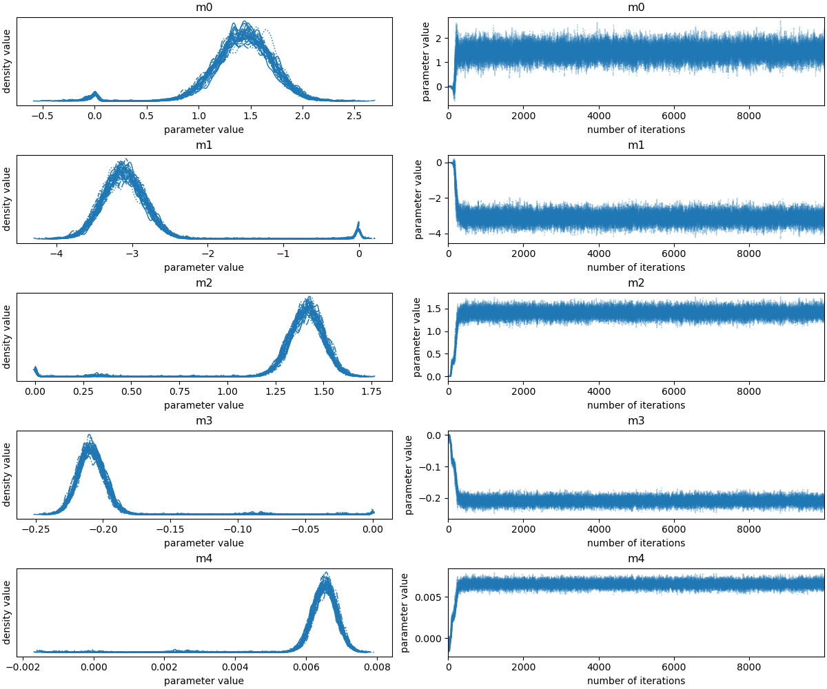
Post-sampling analysis#
By default the raw sampler resulting object is attached to cofi’s
inversion result.
Optionally, you can convert that into an arviz data structure to
have access to a range of analysis functions. (See more details in
arviz
documentation).
import arviz as az

labels = ["m0", "m1", "m2","m3","m4"]

sampler = inv_result_3.sampler
az_idata = az.from_emcee(sampler, var_names=labels)
# az_idata = inv_result_3.to_arviz()      # alternatively
az_idata.get("posterior")
# a standard `trace` plot
axes = az.plot_trace(az_idata, backend_kwargs={"constrained_layout":True});

# add legends
for i, axes_pair in enumerate(axes):
    ax1 = axes_pair[0]
    ax2 = axes_pair[1]
    #ax1.axvline(true_model[i], linestyle='dotted', color='red')
    ax1.set_xlabel("parameter value")
    ax1.set_ylabel("density value")
    ax2.set_xlabel("number of iterations")
    ax2.set_ylabel("parameter value")
#tau = sampler.get_autocorr_time()
#print(f"autocorrelation time: {tau}")
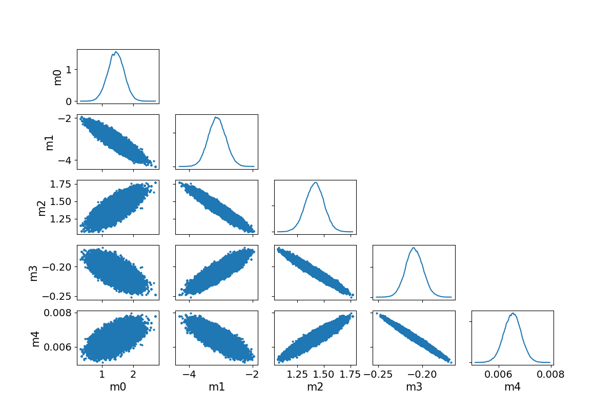
# a Corner plot

fig, axes = plt.subplots(nparams, nparams, figsize=(12,8))

if(True): # if we are plotting the model ensemble use this
    az.plot_pair(
        az_idata.sel(draw=slice(300,None)),
        marginals=True,
        #reference_values=dict(zip([f"m{i}" for i in range(4)], true_model.tolist())),
        ax=axes,
    );
else: # if we wish to plot a kernel density plot then use this option
    az.plot_pair(
        az_idata.sel(draw=slice(300,None)),
        marginals=True,
        #reference_values=dict(zip([f"m{i}" for i in range(4)], true_model.tolist())),
        kind="kde",
        kde_kwargs={
            "hdi_probs": [0.3, 0.6, 0.9],  # Plot 30%, 60% and 90% HDI contours
            "contourf_kwargs": {"cmap": "Blues"},
        },
        ax=axes,
    );
/home/jiawen/opt/mambaforge/envs/cofi_dev/lib/python3.10/site-packages/arviz/plots/pairplot.py:232: FutureWarning: The return type of `Dataset.dims` will be changed to return a set of dimension names in future, in order to be more consistent with `DataArray.dims`. To access a mapping from dimension names to lengths, please use `Dataset.sizes`.
  gridsize = int(dataset.dims["draw"] ** 0.35)
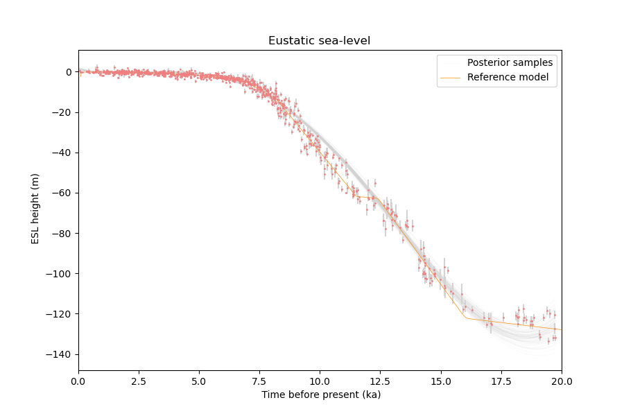
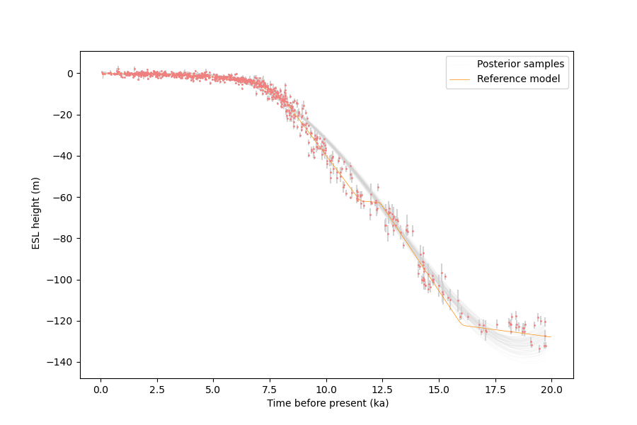
Now we plot the predicted curves for the posterior ensemble of solutions.
flat_samples = sampler.get_chain(discard=300, thin=30, flat=True)
inds = np.random.randint(len(flat_samples), size=100) # get a random selection from posterior ensemble

plot_data(title="Eustatic sea-level")
plt.xlim(0,maxtime)
plot_models(flat_samples[inds],color="lightgrey")
plot_model(ref_x,ref_y, "Reference model", color="darkorange")
#plt.xlim(15,20.)
#plt.ylim(-140,-100)
Expected values, credible intervals and model covariance matrix from the ensemble#
print("\n Expected value and 95% credible intervals ")
for i in range(ndim):
    mcmc = np.percentile(flat_samples[:, i], [5, 50, 95])
    print(" {} {:7.3f} [{:7.3f}, {:7.3f}]".format(labels[i],mcmc[1],mcmc[0],mcmc[2]))
Expected value and 95% credible intervals
m0   1.443 [  1.013,   1.860]
m1  -3.116 [ -3.555,  -2.662]
m2   1.415 [  1.273,   1.552]
m3  -0.209 [ -0.225,  -0.193]
m4   0.007 [  0.006,   0.007]
CMpost = np.cov(flat_samples.T)
CM_std= np.std(flat_samples,axis=0)
print('Posterior model covariance matrix\n',CMpost)
print('\n Posterior estimate of model standard deviations in each parameter')
for i in range(ndim):
    print("    {} {:7.4f}".format(labels[i],CM_std[i]))
Posterior model covariance matrix
 [[ 6.61998057e-02 -6.22285505e-02  1.66044648e-02 -1.60072353e-03
   4.76124752e-05]
 [-6.22285505e-02  7.40607509e-02 -2.22504836e-02  2.31006440e-03
  -7.17313742e-05]
 [ 1.66044648e-02 -2.22504836e-02  7.32465299e-03 -8.12350348e-04
   2.62347880e-05]
 [-1.60072353e-03  2.31006440e-03 -8.12350348e-04  9.49930555e-05
  -3.17120906e-06]
 [ 4.76124752e-05 -7.17313742e-05  2.62347880e-05 -3.17120906e-06
   1.08679748e-07]]

 Posterior estimate of model standard deviations in each parameter
    m0  0.2573
    m1  0.2721
    m2  0.0856
    m3  0.0097
    m4  0.0003
Challenge - Change the prior model bounds#
Replace the previous prior bounds to new values
The original uniform bounds had
\({\mathbf l}^T = (-10.,-10.,-10.,-10.)\), and \({\mathbf u}^T = (10.,10.,10.,10.)\).
Lets replace with
\({\mathbf l}^T = (-0.5,-10.,-10.,-10.)\), and \({\mathbf u}^T = (0.5,10.,10.,10.)\).
We have only changed the bounds of the first parameter. However since the true value of constant term was 6, these bounds are now inconsistent with the true model.
What does this do to the posterior distribution?
Start from the code template below:
m_lower_bound = <CHANGE ME>             # lower bound for uniform prior
m_upper_bound = <CHANGE ME>             # upper bound for uniform prior

def log_prior(model):    # uniform distribution
    for i in range(len(m_lower_bound)):
        if model[i] < m_lower_bound[i] or model[i] > m_upper_bound[i]: return -np.inf
    return 0.0 # model lies within bounds -> return log(1)

######## CoFI BaseProblem - update information
inv_problem.set_log_prior(log_prior)

######## CoFI Inversion - run it
inv_4 = Inversion(inv_problem, inv_options_3)
inv_result_4 = inv_4.run()

flat_samples = inv_result_4.sampler.get_chain(discard=300, thin=30, flat=True)
inds = np.random.randint(len(flat_samples), size=100) # get a random selection from posterior ensemble

print("Resulting samples with prior model lower bounds of <CHANGE ME>, upper bounds of <CHANGE ME>")
plot_data()
plot_models(flat_samples[inds])
plot_model(x, true_y, "True model", color="darkorange")
# Copy the template above, Replace <CHANGE ME> with your answer
#@title Solution

m_lower_bound = np.array([-1.0,-10,-10,-10])             # lower bound for uniform prior
m_upper_bound = np.array([1.0,10,10,10])                 # upper bound for uniform prior

def log_prior(model):    # uniform distribution
    for i in range(len(m_lower_bound)):
        if model[i] < m_lower_bound[i] or model[i] > m_upper_bound[i]: return -np.inf
    return 0.0 # model lies within bounds -> return log(1)

######## CoFI BaseProblem - update information
inv_problem.set_log_prior(log_prior)

######## CoFI Inversion - run it
inv_4 = Inversion(inv_problem, inv_options_3)
inv_result_4 = inv_4.run()

flat_samples = inv_result_4.sampler.get_chain(discard=300, thin=30, flat=True)
inds = np.random.randint(len(flat_samples), size=100) # get a random selection from posterior ensemble

print("Resulting samples with prior model lower bounds of [-1,-10,-10,-10], upper bounds of [2,10,10,10]")
plot_data()
plot_models(flat_samples[inds],color="lightgrey")
plot_model(ref_x, ref_y, "Reference model", color="darkorange")
  0%|          | 0/10000 [00:00<?, ?it/s]
  0%|          | 33/10000 [00:00<00:30, 326.45it/s]
  1%|          | 67/10000 [00:00<00:30, 329.68it/s]
  1%|          | 101/10000 [00:00<00:29, 331.34it/s]
  1%|▏         | 135/10000 [00:00<00:29, 332.05it/s]
  2%|▏         | 169/10000 [00:00<00:29, 332.18it/s]
  2%|▏         | 203/10000 [00:00<00:29, 332.12it/s]
  2%|▏         | 238/10000 [00:00<00:28, 336.65it/s]
  3%|▎         | 275/10000 [00:00<00:28, 345.07it/s]
  3%|▎         | 312/10000 [00:00<00:27, 351.74it/s]
  3%|▎         | 349/10000 [00:01<00:27, 356.89it/s]
  4%|▍         | 386/10000 [00:01<00:26, 359.55it/s]
  4%|▍         | 423/10000 [00:01<00:26, 361.54it/s]
  5%|▍         | 460/10000 [00:01<00:27, 352.40it/s]
  5%|▍         | 496/10000 [00:01<00:33, 284.53it/s]
  5%|▌         | 527/10000 [00:01<00:39, 237.71it/s]
  6%|▌         | 556/10000 [00:01<00:38, 244.79it/s]
  6%|▌         | 583/10000 [00:01<00:45, 207.57it/s]
  6%|▌         | 619/10000 [00:02<00:38, 241.06it/s]
  7%|▋         | 656/10000 [00:02<00:34, 270.28it/s]
  7%|▋         | 693/10000 [00:02<00:31, 294.40it/s]
  7%|▋         | 731/10000 [00:02<00:29, 315.66it/s]
  8%|▊         | 769/10000 [00:02<00:27, 332.25it/s]
  8%|▊         | 807/10000 [00:02<00:26, 345.05it/s]
  8%|▊         | 845/10000 [00:02<00:25, 353.02it/s]
  9%|▉         | 882/10000 [00:02<00:25, 356.54it/s]
  9%|▉         | 920/10000 [00:02<00:25, 361.91it/s]
 10%|▉         | 957/10000 [00:03<00:25, 358.14it/s]
 10%|▉         | 994/10000 [00:03<00:24, 360.48it/s]
 10%|█         | 1032/10000 [00:03<00:24, 365.09it/s]
 11%|█         | 1069/10000 [00:03<00:27, 329.03it/s]
 11%|█         | 1103/10000 [00:03<00:27, 325.50it/s]
 11%|█▏        | 1140/10000 [00:03<00:26, 337.49it/s]
 12%|█▏        | 1177/10000 [00:03<00:25, 345.84it/s]
 12%|█▏        | 1214/10000 [00:03<00:24, 351.52it/s]
 13%|█▎        | 1251/10000 [00:03<00:24, 356.23it/s]
 13%|█▎        | 1288/10000 [00:03<00:24, 358.80it/s]
 13%|█▎        | 1325/10000 [00:04<00:24, 360.13it/s]
 14%|█▎        | 1363/10000 [00:04<00:23, 364.25it/s]
 14%|█▍        | 1400/10000 [00:04<00:23, 365.37it/s]
 14%|█▍        | 1437/10000 [00:04<00:24, 355.99it/s]
 15%|█▍        | 1474/10000 [00:04<00:23, 358.96it/s]
 15%|█▌        | 1510/10000 [00:04<00:26, 315.96it/s]
 15%|█▌        | 1543/10000 [00:04<00:26, 316.21it/s]
 16%|█▌        | 1576/10000 [00:04<00:28, 300.55it/s]
 16%|█▌        | 1607/10000 [00:04<00:29, 281.67it/s]
 16%|█▋        | 1636/10000 [00:05<00:29, 282.44it/s]
 17%|█▋        | 1665/10000 [00:05<00:34, 244.61it/s]
 17%|█▋        | 1691/10000 [00:05<00:35, 236.63it/s]
 17%|█▋        | 1728/10000 [00:05<00:30, 269.98it/s]
 18%|█▊        | 1757/10000 [00:05<00:31, 264.16it/s]
 18%|█▊        | 1785/10000 [00:05<00:32, 255.18it/s]
 18%|█▊        | 1812/10000 [00:05<00:31, 258.31it/s]
 18%|█▊        | 1839/10000 [00:05<00:34, 235.79it/s]
 19%|█▊        | 1864/10000 [00:06<00:35, 232.41it/s]
 19%|█▉        | 1901/10000 [00:06<00:30, 267.35it/s]
 19%|█▉        | 1938/10000 [00:06<00:27, 294.79it/s]
 20%|█▉        | 1976/10000 [00:06<00:25, 317.47it/s]
 20%|██        | 2009/10000 [00:06<00:25, 314.10it/s]
 20%|██        | 2046/10000 [00:06<00:24, 329.03it/s]
 21%|██        | 2083/10000 [00:06<00:23, 340.39it/s]
 21%|██        | 2118/10000 [00:06<00:24, 328.26it/s]
 22%|██▏       | 2156/10000 [00:06<00:22, 341.77it/s]
 22%|██▏       | 2193/10000 [00:06<00:22, 347.68it/s]
 22%|██▏       | 2230/10000 [00:07<00:21, 353.64it/s]
 23%|██▎       | 2268/10000 [00:07<00:21, 360.07it/s]
 23%|██▎       | 2306/10000 [00:07<00:21, 364.22it/s]
 23%|██▎       | 2345/10000 [00:07<00:20, 369.23it/s]
 24%|██▍       | 2383/10000 [00:07<00:20, 369.96it/s]
 24%|██▍       | 2421/10000 [00:07<00:20, 372.51it/s]
 25%|██▍       | 2459/10000 [00:07<00:20, 372.95it/s]
 25%|██▍       | 2497/10000 [00:07<00:20, 369.99it/s]
 25%|██▌       | 2535/10000 [00:07<00:24, 308.14it/s]
 26%|██▌       | 2572/10000 [00:08<00:23, 322.34it/s]
 26%|██▌       | 2609/10000 [00:08<00:22, 334.97it/s]
 26%|██▋       | 2647/10000 [00:08<00:21, 345.09it/s]
 27%|██▋       | 2685/10000 [00:08<00:20, 353.28it/s]
 27%|██▋       | 2724/10000 [00:08<00:20, 361.44it/s]
 28%|██▊       | 2762/10000 [00:08<00:19, 365.54it/s]
 28%|██▊       | 2799/10000 [00:08<00:19, 363.52it/s]
 28%|██▊       | 2836/10000 [00:08<00:19, 363.09it/s]
 29%|██▊       | 2873/10000 [00:08<00:23, 307.33it/s]
 29%|██▉       | 2910/10000 [00:09<00:21, 322.37it/s]
 29%|██▉       | 2946/10000 [00:09<00:22, 315.26it/s]
 30%|██▉       | 2982/10000 [00:09<00:21, 326.37it/s]
 30%|███       | 3018/10000 [00:09<00:20, 335.13it/s]
 31%|███       | 3054/10000 [00:09<00:20, 341.61it/s]
 31%|███       | 3089/10000 [00:09<00:20, 343.59it/s]
 31%|███       | 3124/10000 [00:09<00:20, 343.40it/s]
 32%|███▏      | 3162/10000 [00:09<00:19, 352.08it/s]
 32%|███▏      | 3198/10000 [00:09<00:22, 305.24it/s]
 32%|███▏      | 3234/10000 [00:10<00:21, 319.67it/s]
 33%|███▎      | 3268/10000 [00:10<00:31, 215.64it/s]
 33%|███▎      | 3295/10000 [00:10<00:32, 209.38it/s]
 33%|███▎      | 3331/10000 [00:10<00:27, 240.49it/s]
 34%|███▎      | 3367/10000 [00:10<00:24, 267.17it/s]
 34%|███▍      | 3404/10000 [00:10<00:22, 291.79it/s]
 34%|███▍      | 3440/10000 [00:10<00:21, 307.01it/s]
 35%|███▍      | 3473/10000 [00:11<00:27, 236.32it/s]
 35%|███▌      | 3501/10000 [00:11<00:30, 216.57it/s]
 35%|███▌      | 3528/10000 [00:11<00:28, 227.90it/s]
 36%|███▌      | 3564/10000 [00:11<00:24, 258.15it/s]
 36%|███▌      | 3601/10000 [00:11<00:22, 285.51it/s]
 36%|███▋      | 3638/10000 [00:11<00:20, 307.50it/s]
 37%|███▋      | 3675/10000 [00:11<00:19, 323.94it/s]
 37%|███▋      | 3711/10000 [00:11<00:18, 333.98it/s]
 37%|███▋      | 3748/10000 [00:11<00:18, 342.25it/s]
 38%|███▊      | 3785/10000 [00:12<00:17, 347.83it/s]
 38%|███▊      | 3822/10000 [00:12<00:17, 353.59it/s]
 39%|███▊      | 3860/10000 [00:12<00:17, 360.26it/s]
 39%|███▉      | 3897/10000 [00:12<00:16, 360.86it/s]
 39%|███▉      | 3934/10000 [00:12<00:20, 300.34it/s]
 40%|███▉      | 3969/10000 [00:12<00:19, 312.16it/s]
 40%|████      | 4006/10000 [00:12<00:18, 326.19it/s]
 40%|████      | 4040/10000 [00:12<00:21, 278.13it/s]
 41%|████      | 4070/10000 [00:13<00:22, 265.94it/s]
 41%|████      | 4098/10000 [00:13<00:34, 172.73it/s]
 41%|████      | 4121/10000 [00:13<00:37, 155.00it/s]
 41%|████▏     | 4140/10000 [00:13<00:36, 161.06it/s]
 42%|████▏     | 4159/10000 [00:13<00:36, 158.98it/s]
 42%|████▏     | 4177/10000 [00:13<00:35, 163.23it/s]
 42%|████▏     | 4198/10000 [00:13<00:33, 174.04it/s]
 42%|████▏     | 4217/10000 [00:14<00:34, 169.19it/s]
 42%|████▏     | 4235/10000 [00:14<00:49, 116.63it/s]
 43%|████▎     | 4251/10000 [00:14<00:46, 124.83it/s]
 43%|████▎     | 4281/10000 [00:14<00:35, 163.00it/s]
 43%|████▎     | 4303/10000 [00:14<00:32, 176.63it/s]
 43%|████▎     | 4324/10000 [00:14<00:30, 184.00it/s]
 43%|████▎     | 4345/10000 [00:14<00:37, 151.41it/s]
 44%|████▍     | 4383/10000 [00:15<00:27, 203.18it/s]
 44%|████▍     | 4411/10000 [00:15<00:25, 221.04it/s]
 44%|████▍     | 4441/10000 [00:15<00:23, 240.20it/s]
 45%|████▍     | 4467/10000 [00:15<00:22, 244.00it/s]
 45%|████▌     | 4500/10000 [00:15<00:20, 266.71it/s]
 45%|████▌     | 4538/10000 [00:15<00:18, 296.59it/s]
 46%|████▌     | 4576/10000 [00:15<00:17, 319.02it/s]
 46%|████▌     | 4609/10000 [00:15<00:21, 254.43it/s]
 46%|████▋     | 4648/10000 [00:16<00:18, 286.60it/s]
 47%|████▋     | 4687/10000 [00:16<00:16, 312.63it/s]
 47%|████▋     | 4721/10000 [00:16<00:16, 315.31it/s]
 48%|████▊     | 4760/10000 [00:16<00:15, 334.79it/s]
 48%|████▊     | 4797/10000 [00:16<00:15, 343.41it/s]
 48%|████▊     | 4835/10000 [00:16<00:14, 353.63it/s]
 49%|████▊     | 4872/10000 [00:16<00:14, 357.70it/s]
 49%|████▉     | 4911/10000 [00:16<00:13, 364.93it/s]
 49%|████▉     | 4948/10000 [00:16<00:13, 366.38it/s]
 50%|████▉     | 4986/10000 [00:16<00:13, 370.17it/s]
 50%|█████     | 5024/10000 [00:17<00:14, 350.32it/s]
 51%|█████     | 5063/10000 [00:17<00:13, 358.95it/s]
 51%|█████     | 5100/10000 [00:17<00:15, 311.32it/s]
 51%|█████▏    | 5139/10000 [00:17<00:14, 329.61it/s]
 52%|█████▏    | 5177/10000 [00:17<00:14, 341.44it/s]
 52%|█████▏    | 5216/10000 [00:17<00:13, 352.33it/s]
 53%|█████▎    | 5253/10000 [00:17<00:13, 357.02it/s]
 53%|█████▎    | 5290/10000 [00:17<00:13, 356.78it/s]
 53%|█████▎    | 5329/10000 [00:17<00:12, 364.58it/s]
 54%|█████▎    | 5367/10000 [00:18<00:12, 368.88it/s]
 54%|█████▍    | 5405/10000 [00:18<00:12, 371.30it/s]
 54%|█████▍    | 5443/10000 [00:18<00:12, 371.28it/s]
 55%|█████▍    | 5482/10000 [00:18<00:12, 374.25it/s]
 55%|█████▌    | 5520/10000 [00:18<00:11, 375.31it/s]
 56%|█████▌    | 5558/10000 [00:18<00:11, 374.00it/s]
 56%|█████▌    | 5596/10000 [00:18<00:11, 375.22it/s]
 56%|█████▋    | 5634/10000 [00:18<00:11, 374.91it/s]
 57%|█████▋    | 5672/10000 [00:18<00:11, 374.10it/s]
 57%|█████▋    | 5712/10000 [00:18<00:11, 380.23it/s]
 58%|█████▊    | 5751/10000 [00:19<00:11, 379.99it/s]
 58%|█████▊    | 5790/10000 [00:19<00:11, 378.27it/s]
 58%|█████▊    | 5828/10000 [00:19<00:11, 377.19it/s]
 59%|█████▊    | 5867/10000 [00:19<00:10, 378.28it/s]
 59%|█████▉    | 5905/10000 [00:19<00:10, 377.70it/s]
 59%|█████▉    | 5943/10000 [00:19<00:10, 376.46it/s]
 60%|█████▉    | 5981/10000 [00:19<00:10, 373.81it/s]
 60%|██████    | 6019/10000 [00:19<00:10, 370.23it/s]
 61%|██████    | 6057/10000 [00:19<00:10, 368.45it/s]
 61%|██████    | 6094/10000 [00:19<00:10, 367.37it/s]
 61%|██████▏   | 6132/10000 [00:20<00:10, 368.95it/s]
 62%|██████▏   | 6170/10000 [00:20<00:10, 370.07it/s]
 62%|██████▏   | 6208/10000 [00:20<00:10, 370.16it/s]
 62%|██████▏   | 6247/10000 [00:20<00:10, 374.42it/s]
 63%|██████▎   | 6286/10000 [00:20<00:09, 376.84it/s]
 63%|██████▎   | 6324/10000 [00:20<00:09, 377.17it/s]
 64%|██████▎   | 6362/10000 [00:20<00:09, 377.44it/s]
 64%|██████▍   | 6401/10000 [00:20<00:09, 379.76it/s]
 64%|██████▍   | 6440/10000 [00:20<00:09, 380.14it/s]
 65%|██████▍   | 6479/10000 [00:20<00:09, 379.22it/s]
 65%|██████▌   | 6517/10000 [00:21<00:09, 378.63it/s]
 66%|██████▌   | 6556/10000 [00:21<00:09, 379.37it/s]
 66%|██████▌   | 6594/10000 [00:21<00:09, 376.89it/s]
 66%|██████▋   | 6632/10000 [00:21<00:08, 375.29it/s]
 67%|██████▋   | 6670/10000 [00:21<00:08, 375.17it/s]
 67%|██████▋   | 6708/10000 [00:21<00:08, 375.86it/s]
 67%|██████▋   | 6746/10000 [00:21<00:08, 375.65it/s]
 68%|██████▊   | 6784/10000 [00:21<00:08, 375.63it/s]
 68%|██████▊   | 6822/10000 [00:21<00:08, 376.78it/s]
 69%|██████▊   | 6860/10000 [00:21<00:08, 371.38it/s]
 69%|██████▉   | 6898/10000 [00:22<00:08, 373.20it/s]
 69%|██████▉   | 6936/10000 [00:22<00:08, 373.67it/s]
 70%|██████▉   | 6974/10000 [00:22<00:08, 375.25it/s]
 70%|███████   | 7012/10000 [00:22<00:07, 375.50it/s]
 70%|███████   | 7050/10000 [00:22<00:07, 375.51it/s]
 71%|███████   | 7088/10000 [00:22<00:08, 343.09it/s]
 71%|███████▏  | 7126/10000 [00:22<00:08, 352.63it/s]
 72%|███████▏  | 7164/10000 [00:22<00:07, 359.54it/s]
 72%|███████▏  | 7202/10000 [00:22<00:07, 364.92it/s]
 72%|███████▏  | 7241/10000 [00:23<00:07, 370.47it/s]
 73%|███████▎  | 7279/10000 [00:23<00:07, 369.01it/s]
 73%|███████▎  | 7317/10000 [00:23<00:07, 370.44it/s]
 74%|███████▎  | 7355/10000 [00:23<00:07, 371.59it/s]
 74%|███████▍  | 7393/10000 [00:23<00:06, 373.22it/s]
 74%|███████▍  | 7432/10000 [00:23<00:06, 376.27it/s]
 75%|███████▍  | 7471/10000 [00:23<00:06, 380.21it/s]
 75%|███████▌  | 7510/10000 [00:23<00:06, 377.88it/s]
 75%|███████▌  | 7548/10000 [00:23<00:06, 375.14it/s]
 76%|███████▌  | 7586/10000 [00:23<00:06, 374.81it/s]
 76%|███████▌  | 7624/10000 [00:24<00:06, 375.14it/s]
 77%|███████▋  | 7662/10000 [00:24<00:06, 373.90it/s]
 77%|███████▋  | 7700/10000 [00:24<00:06, 374.53it/s]
 77%|███████▋  | 7739/10000 [00:24<00:05, 376.93it/s]
 78%|███████▊  | 7778/10000 [00:24<00:05, 379.43it/s]
 78%|███████▊  | 7816/10000 [00:24<00:05, 378.10it/s]
 79%|███████▊  | 7854/10000 [00:24<00:05, 378.19it/s]
 79%|███████▉  | 7893/10000 [00:24<00:05, 379.54it/s]
 79%|███████▉  | 7931/10000 [00:24<00:05, 379.41it/s]
 80%|███████▉  | 7969/10000 [00:24<00:05, 379.32it/s]
 80%|████████  | 8007/10000 [00:25<00:05, 379.07it/s]
 80%|████████  | 8045/10000 [00:25<00:05, 378.13it/s]
 81%|████████  | 8083/10000 [00:25<00:05, 378.63it/s]
 81%|████████  | 8121/10000 [00:25<00:04, 376.99it/s]
 82%|████████▏ | 8159/10000 [00:25<00:04, 372.74it/s]
 82%|████████▏ | 8197/10000 [00:25<00:04, 374.50it/s]
 82%|████████▏ | 8235/10000 [00:25<00:04, 374.68it/s]
 83%|████████▎ | 8274/10000 [00:25<00:04, 377.55it/s]
 83%|████████▎ | 8312/10000 [00:25<00:04, 377.81it/s]
 84%|████████▎ | 8350/10000 [00:25<00:04, 377.60it/s]
 84%|████████▍ | 8388/10000 [00:26<00:04, 378.01it/s]
 84%|████████▍ | 8428/10000 [00:26<00:04, 381.88it/s]
 85%|████████▍ | 8467/10000 [00:26<00:04, 380.51it/s]
 85%|████████▌ | 8506/10000 [00:26<00:03, 382.70it/s]
 85%|████████▌ | 8545/10000 [00:26<00:03, 381.57it/s]
 86%|████████▌ | 8584/10000 [00:26<00:03, 380.26it/s]
 86%|████████▌ | 8623/10000 [00:26<00:03, 379.57it/s]
 87%|████████▋ | 8661/10000 [00:26<00:03, 377.28it/s]
 87%|████████▋ | 8699/10000 [00:26<00:03, 376.60it/s]
 87%|████████▋ | 8737/10000 [00:26<00:03, 377.05it/s]
 88%|████████▊ | 8775/10000 [00:27<00:03, 376.62it/s]
 88%|████████▊ | 8813/10000 [00:27<00:03, 374.08it/s]
 89%|████████▊ | 8851/10000 [00:27<00:03, 374.80it/s]
 89%|████████▉ | 8890/10000 [00:27<00:02, 378.48it/s]
 89%|████████▉ | 8929/10000 [00:27<00:02, 379.40it/s]
 90%|████████▉ | 8967/10000 [00:27<00:02, 378.23it/s]
 90%|█████████ | 9005/10000 [00:27<00:02, 377.92it/s]
 90%|█████████ | 9043/10000 [00:27<00:02, 370.64it/s]
 91%|█████████ | 9081/10000 [00:27<00:02, 372.50it/s]
 91%|█████████ | 9119/10000 [00:28<00:02, 370.27it/s]
 92%|█████████▏| 9157/10000 [00:28<00:02, 372.60it/s]
 92%|█████████▏| 9195/10000 [00:28<00:02, 363.72it/s]
 92%|█████████▏| 9234/10000 [00:28<00:02, 370.82it/s]
 93%|█████████▎| 9272/10000 [00:28<00:01, 371.94it/s]
 93%|█████████▎| 9310/10000 [00:28<00:01, 373.14it/s]
 93%|█████████▎| 9349/10000 [00:28<00:01, 376.07it/s]
 94%|█████████▍| 9387/10000 [00:28<00:01, 376.59it/s]
 94%|█████████▍| 9425/10000 [00:28<00:01, 375.38it/s]
 95%|█████████▍| 9464/10000 [00:28<00:01, 379.40it/s]
 95%|█████████▌| 9503/10000 [00:29<00:01, 380.25it/s]
 95%|█████████▌| 9542/10000 [00:29<00:01, 379.59it/s]
 96%|█████████▌| 9581/10000 [00:29<00:01, 381.21it/s]
 96%|█████████▌| 9620/10000 [00:29<00:01, 379.73it/s]
 97%|█████████▋| 9659/10000 [00:29<00:00, 381.14it/s]
 97%|█████████▋| 9698/10000 [00:29<00:00, 378.60it/s]
 97%|█████████▋| 9736/10000 [00:29<00:00, 378.13it/s]
 98%|█████████▊| 9774/10000 [00:29<00:00, 377.63it/s]
 98%|█████████▊| 9812/10000 [00:29<00:00, 378.22it/s]
 98%|█████████▊| 9850/10000 [00:29<00:00, 377.38it/s]
 99%|█████████▉| 9888/10000 [00:30<00:00, 374.94it/s]
 99%|█████████▉| 9926/10000 [00:30<00:00, 373.79it/s]
100%|█████████▉| 9964/10000 [00:30<00:00, 274.66it/s]
100%|█████████▉| 9999/10000 [00:30<00:00, 291.70it/s]
100%|██████████| 10000/10000 [00:30<00:00, 328.00it/s]
Resulting samples with prior model lower bounds of [-1,-10,-10,-10], upper bounds of [2,10,10,10]
Is there much change to the posterior distribution?
Watermark#
watermark_list = ["cofi", "numpy", "scipy", "matplotlib", "emcee", "arviz"]
for pkg in watermark_list:
    pkg_var = __import__(pkg)
    print(pkg, getattr(pkg_var, "__version__"))
cofi 0.2.7
numpy 1.24.4
scipy 1.12.0
matplotlib 3.8.3
emcee 3.1.4
arviz 0.17.0
sphinx_gallery_thumbnail_number = -1
Total running time of the script: (1 minutes 12.274 seconds)

