Seismic Wave Tomography via Fast Marching

If you are running this notebook locally, make sure you’ve followed steps here to set up the environment. (This environment.yml file specifies a list of packages required to run the notebooks)

0. Import modules

# -------------------------------------------------------- #
#                                                          #
#     Uncomment below to set up environment on "colab"     #
#                                                          #
# -------------------------------------------------------- #

# !pip install -U cofi geo-espresso
# !git clone https://github.com/inlab-geo/cofi-examples.git
# %cd cofi-examples/examples/fmm_tomography

import numpy as np
import matplotlib.pyplot as plt
import pprint

import cofi
import espresso

In this notebook, we use cofi to run a seismic wave tomography example, in which the forward calculation is based on the Fast Marching Fortran code by Nick Rawlinson. The Fast Marching code is wrapped in package espresso.

Theoretical background

# display theory on travel time tomography
from IPython.display import display, Markdown

with open("../../theory/geo_travel_time_tomography.md", "r") as f:
    content = f.read()

display(Markdown(content))

<IPython.core.display.Markdown object>

In this notebook we form and solve a travel time tomography problem using model damping and 2nd derivative smoothing. For forward modelling, a fast marching wave front tracker is used, utilizing the Fast Marching Fortran code within the package `FMTOMO <http://iearth.edu.au/codes/FMTOMO/>`__ by Nick Rawlinson.

Problem setup

Before we starting working with cofi, let’s get familiar with the problem itself.

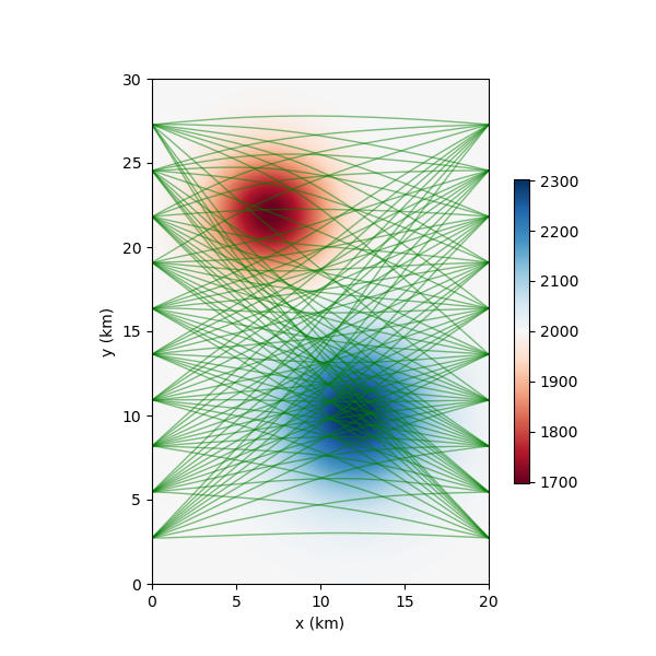
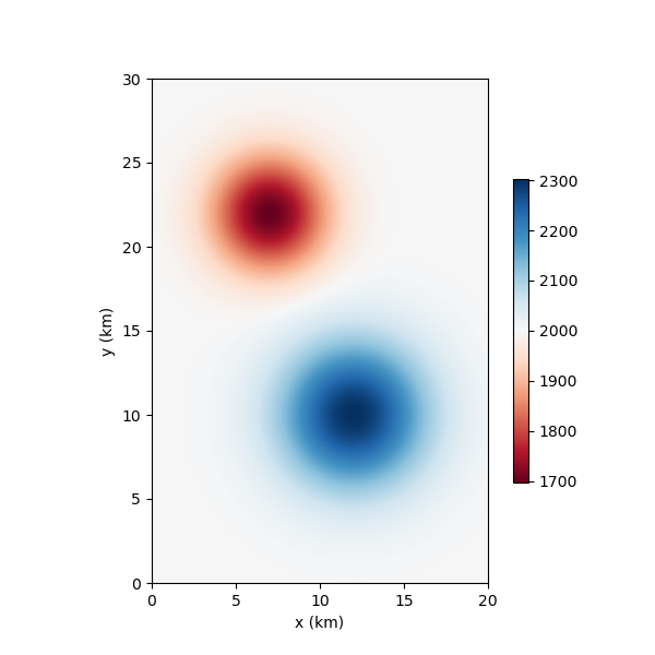
Below is a plot of the true model and the paths generated from this model. As you can see, there are two anomalies, one with lower velocity (red, top left) and the other with higher velocity (blue, bottom right).

fmm = espresso.FmmTomography()

fmm.plot_model(fmm.good_model, with_paths=True);

 New data set has:
 10  receivers
 10  sources
 100  travel times
 Range of travel times:  0.008911182496368759 0.0153757024856463
 Mean travel time: 0.01085811731230709
Trying to fix now...
Execute permission given to fm2dss.o.

<Axes: xlabel='x (km)', ylabel='y (km)'>

pprint.pprint(fmm.metadata)

{'author_names': ['Nick Rawlinson', 'Malcolm Sambridge'],
 'citations': [('Rawlinson, N., de Kool, M. and Sambridge, M., 2006. Seismic '
                'wavefront tracking in 3-D heterogeneous media: applications '
                'with multiple data classes, Explor. Geophys., 37, 322-330.',
                ''),
               ('Rawlinson, N. and Urvoy, M., 2006. Simultaneous inversion of '
                'active and passive source datasets for 3-D seismic structure '
                'with application to Tasmania, Geophys. Res. Lett., 33 L24313',
                '10.1029/2006GL028105'),
               ('de Kool, M., Rawlinson, N. and Sambridge, M. 2006. A '
                'practical grid based method for tracking multiple refraction '
                'and reflection phases in 3D heterogeneous media, Geophys. J. '
                'Int., 167, 253-270',
                ''),
               ('Saygin, E. 2007. Seismic receiver and noise correlation based '
                'studies in Australia, PhD thesis, Australian National '
                'University.',
                '10.25911/5d7a2d1296f96')],
 'contact_email': 'Malcolm.Sambridge@anu.edu.au',
 'contact_name': 'Malcolm Sambridge',
 'linked_sites': [('Software published on iEarth',
                   'http://iearth.edu.au/codes/FMTOMO/')],
 'problem_short_description': 'The wave front tracker routines solves boundary '
                              'value ray tracing problems into 2D '
                              'heterogeneous wavespeed media, defined by '
                              'continuously varying velocity model calculated '
                              'by 2D cubic B-splines.',
 'problem_title': 'Fast Marching Wave Front Tracking'}

1. Define the problem

# get problem information from  espresso FmmTomography
model_size = fmm.model_size         # number of model parameters
model_shape = fmm.model_shape       # 2D spatial grids
data_size = fmm.data_size           # number of data points
ref_start_slowness = fmm.starting_model

# define CoFI BaseProblem
fmm_problem = cofi.BaseProblem()
fmm_problem.set_initial_model(ref_start_slowness)

# add regularization: damping + smoothing
damping_factor = 50
smoothing_factor = 5e3
reg_damping = damping_factor * cofi.utils.QuadraticReg(
    model_shape=model_shape,
    weighting_matrix="damping",
    reference_model=ref_start_slowness
)
reg_smoothing = smoothing_factor * cofi.utils.QuadraticReg(
    model_shape=model_shape,
    weighting_matrix="smoothing"
)
reg = reg_damping + reg_smoothing

def objective_func(slowness, reg, sigma, reduce_data=None):  # reduce_data=(idx_from, idx_to)
    if reduce_data is None: idx_from, idx_to = (0, fmm.data_size)
    else: idx_from, idx_to = reduce_data
    ttimes = fmm.forward(slowness)
    residual = fmm.data[idx_from:idx_to] - ttimes[idx_from:idx_to]
    data_misfit = residual.T @ residual / sigma**2
    model_reg = reg(slowness)
    return  data_misfit + model_reg

def gradient(slowness, reg, sigma, reduce_data=None):       # reduce_data=(idx_from, idx_to)
    if reduce_data is None: idx_from, idx_to = (0, fmm.data_size)
    else: idx_from, idx_to = reduce_data
    ttimes, A = fmm.forward(slowness, return_jacobian=True)
    ttimes = ttimes[idx_from:idx_to]
    A = A[idx_from:idx_to]
    data_misfit_grad = -2 * A.T @ (fmm.data[idx_from:idx_to] - ttimes) / sigma**2
    model_reg_grad = reg.gradient(slowness)
    return  data_misfit_grad + model_reg_grad

def hessian(slowness, reg, sigma, reduce_data=None):        # reduce_data=(idx_from, idx_to)
    if reduce_data is None: idx_from, idx_to = (0, fmm.data_size)
    else: idx_from, idx_to = reduce_data
    A = fmm.jacobian(slowness)[idx_from:idx_to]
    data_misfit_hess = 2 * A.T @ A / sigma**2
    model_reg_hess = reg.hessian(slowness)
    return data_misfit_hess + model_reg_hess

sigma =  0.00001                   # Noise is 1.0E-4 is ~5% of standard deviation of initial travel time residuals

fmm_problem.set_objective(objective_func, args=[reg, sigma, None])
fmm_problem.set_gradient(gradient, args=[reg, sigma, None])
fmm_problem.set_hessian(hessian, args=[reg, sigma, None])

Review what information is included in the BaseProblem object:

fmm_problem.summary()

=====================================================================
Summary for inversion problem: BaseProblem
=====================================================================
Model shape: (1536,)
---------------------------------------------------------------------
List of functions/properties set by you:
['objective', 'gradient', 'hessian', 'initial_model', 'model_shape']
---------------------------------------------------------------------
List of functions/properties created based on what you have provided:
['hessian_times_vector']
---------------------------------------------------------------------
List of functions/properties that can be further set for the problem:
( not all of these may be relevant to your inversion workflow )
['log_posterior', 'log_posterior_with_blobs', 'log_likelihood', 'log_prior', 'hessian_times_vector', 'residual', 'jacobian', 'jacobian_times_vector', 'data_misfit', 'regularization', 'regularization_matrix', 'forward', 'data', 'data_covariance', 'data_covariance_inv', 'blobs_dtype', 'bounds', 'constraints']

2. Define the inversion options

my_options = cofi.InversionOptions()

# cofi's own simple newton's matrix-based optimization solver
my_options.set_tool("cofi.simple_newton")
my_options.set_params(num_iterations=5, step_length=1, verbose=True)

Review what’s been defined for the inversion we are about to run:

my_options.summary()

=============================
Summary for inversion options
=============================
Solving method: None set
Use `suggest_solving_methods()` to check available solving methods.
-----------------------------
Backend tool: `<class 'cofi.tools._cofi_simple_newton.CoFISimpleNewton'>` - CoFI's own solver - simple Newton's approach (for testing mainly)
References: ['https://en.wikipedia.org/wiki/Newton%27s_method_in_optimization']
Use `suggest_tools()` to check available backend tools.
-----------------------------
Solver-specific parameters:
num_iterations = 5
step_length = 1
verbose = True
Use `suggest_solver_params()` to check required/optional solver-specific parameters.

3. Start an inversion

inv = cofi.Inversion(fmm_problem, my_options)
inv_result = inv.run()
inv_result.summary()

Iteration #0, updated objective function value: 1787.077540309464
Iteration #1, updated objective function value: 121.06987606708411
Iteration #2, updated objective function value: 5.825780480485424
Iteration #3, updated objective function value: 3.671788666773696
Iteration #4, updated objective function value: 1.6075547129972418
============================
Summary for inversion result
============================
SUCCESS
----------------------------
model: [0.00048285 0.00048069 0.00047884 ... 0.00050868 0.000508   0.00050718]
num_iterations: 4
objective_val: 1.6075547129972418
n_obj_evaluations: 6
n_grad_evaluations: 5
n_hess_evaluations: 5

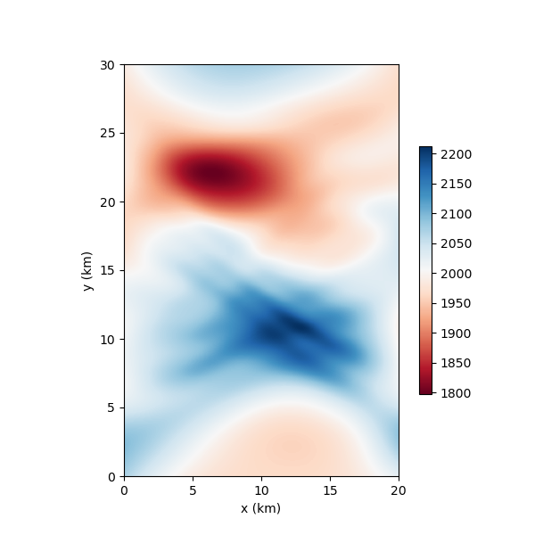
4. Plotting

fmm.plot_model(inv_result.model);            # inverted model
fmm.plot_model(fmm.good_model);       # true model

• 
• 

<Axes: xlabel='x (km)', ylabel='y (km)'>

---

Watermark

watermark_list = ["cofi", "espresso", "numpy", "matplotlib"]
for pkg in watermark_list:
    pkg_var = __import__(pkg)
    print(pkg, getattr(pkg_var, "__version__"))

cofi 0.2.7
espresso 0.3.13
numpy 1.24.4
matplotlib 3.8.3

sphinx_gallery_thumbnail_number = -1